6  Stochastic simulation

The ODE models of Chapter 3 treat concentrations as smooth, continuous quantities. Inside a single cell, however, many molecules are present in tiny numbers: a gene has one or two copies, and a given mRNA may be present as a handful of molecules. Each reaction is then a discrete, random event, and two genetically identical cells in the same environment can hold quite different numbers of a protein. This chapter simulates such systems with Gillespie’s algorithm, and shows how the random fluctuations, or noise, depend on the reactions that produce them.

NoteIn the book

The book deals with deterministic models, and notes that stochastic models, widely simulated with Gillespie’s algorithm, are important when molecule numbers are small (§1.4.3, Modelling paradigms). This chapter fills in that topic. For a fuller treatment, see the reviews by Gillespie (2007) and Raj and Oudenaarden (2008).

6.1 Gillespie’s algorithm

Consider a set of reactions, each with a propensity \(a_j(\mathbf{x})\): the probability per unit time that reaction \(j\) occurs, given the current numbers of molecules \(\mathbf{x}\). For a reaction \(\text{M} \to \emptyset\) with rate constant \(\gamma\), for instance, the propensity is \(\gamma M\), since each of the \(M\) molecules can be degraded. Gillespie’s stochastic simulation algorithm (SSA) generates exact sample paths of such a system (Gillespie 1977):

1. Compute all propensities and their sum, \(a_0 = \sum_j a_j(\mathbf{x})\).
2. Draw the time to the next reaction from an exponential distribution with mean \(1/a_0\): \(\tau = -\ln(r_1)/a_0\), with \(r_1\) uniform on \((0, 1)\).
3. Choose which reaction occurs: reaction \(j\) with probability \(a_j/a_0\).
4. Advance time by \(\tau\), update \(\mathbf{x}\) for that reaction, and repeat.

Both languages have a short implementation of these four steps in the primer’s helper package (sbp.gillespie), which returns the state at a chosen set of times. Here is the Python version; the MATLAB one, in matlab/+sbp/gillespie.m, follows it line by line.

"""Gillespie's stochastic simulation algorithm (SSA), shared by examples."""
import numpy as np


def gillespie(x0, changes, propensities, t_grid, rng):
    """Simulate one trajectory and return the state at the times t_grid.

    x0            initial numbers of molecules (one per species)
    changes       one row per reaction: how each species changes when the
                  reaction fires
    propensities  function of the state x, returning one rate per reaction
    t_grid        increasing times at which to record the state
    rng           a numpy random generator
    """
    changes = np.asarray(changes)
    x = np.array(x0, dtype=float)
    t = 0.0
    out = np.zeros((len(t_grid), len(x)))
    k = 0
    while k < len(t_grid):
        a = propensities(x)
        a0 = a.sum()
        # Time to the next reaction: exponential with mean 1/a0
        tau = rng.exponential(1 / a0) if a0 > 0 else np.inf
        # Record the current state at every grid time before the event
        while k < len(t_grid) and t_grid[k] < t + tau:
            out[k] = x
            k += 1
        t += tau
        if k < len(t_grid):
            # Which reaction: reaction j with probability a_j / a0
            j = np.searchsorted(np.cumsum(a), rng.random() * a0, side="right")
            x += changes[j]
    return out

6.2 Production and degradation of an mRNA

The simplest example is an mRNA made at a constant rate \(k\) and degraded at rate \(\gamma\) per molecule:

\[ \emptyset \xrightarrow{k} \text{M}, \qquad \text{M} \xrightarrow{\gamma M} \emptyset . \]

The ODE model, \(dM/dt = k - \gamma M\), rises smoothly to \(M = k/\gamma\). The stochastic model has a steady state too, but it is a steady distribution: the number of molecules keeps fluctuating, and for this model it follows a Poisson distribution with mean \(k/\gamma\), whose variance is equal to its mean. We take \(k = 10\) per minute and \(\gamma = 1\) per minute, and run the SSA 2000 times.

MATLAB

Core MATLAB only.

%% Stochastic production and degradation of an mRNA
%     0 -> M     at rate k          (transcription)
%     M -> 0     at rate gamma * M  (degradation)
% The deterministic (ODE) model, dM/dt = k - gamma*M, predicts a smooth
% rise to M = k/gamma. With few molecules, each reaction is a random
% event, simulated here with Gillespie's algorithm. At steady state the
% number of molecules follows a Poisson distribution with mean k/gamma.
% Requires: core MATLAB only.

k = 10; gamma = 1;                 % per minute
t_grid = linspace(0, 10, 201);     % minutes
n_runs = 2000;
rng(1);

changes = [+1; -1];
propensities = @(x) [k, gamma * x(1)];

runs = zeros(n_runs, numel(t_grid));
for r = 1:n_runs
    runs(r, :) = sbp.gillespie(0, changes, propensities, t_grid)';
end
final = runs(:, end);
ode = k / gamma * (1 - exp(-gamma * t_grid));

fprintf(['At t = %g min, over %d runs: mean %.3f, variance %.3f ' ...
    '(Poisson: both %g)\n'], t_grid(end), n_runs, mean(final), ...
    var(final, 1), k / gamma);

%% Plot
fig = figure('Position', [100 100 1000 400]);
subplot(1, 2, 1)
colors = [0.122 0.467 0.706; 0.173 0.627 0.173; 0.580 0.404 0.741];
for r = 1:3
    stairs(t_grid, runs(r, :), 'Color', colors(r, :));
    hold on
end
plot(t_grid, mean(runs, 1), '-', 'Color', [1.000 0.498 0.055], ...
    'LineWidth', 2);
plot(t_grid, ode, 'k--', 'LineWidth', 1.5);
ylim([0 25]);
xlabel('Time (min)'); ylabel('Number of mRNA molecules');
legend({'one simulation', '', '', ...
    sprintf('mean of %d simulations', n_runs), 'ODE'}, ...
    'Location', 'northwest', 'Box', 'off');
title('Trajectories');
box off

subplot(1, 2, 2)
m = 0:25;
counts = histcounts(final, -0.5:25.5) / n_runs;
bar(m, counts, 'FaceColor', [0.122 0.467 0.706], 'FaceAlpha', 0.7, ...
    'EdgeColor', 'none');
hold on
lambda = k / gamma;
plot(m, exp(-lambda) * lambda.^m ./ factorial(m), 'o-', ...
    'Color', [1.000 0.498 0.055], 'MarkerSize', 4, ...
    'MarkerFaceColor', [1.000 0.498 0.055]);
ylim([0 0.17]);
xlabel('Number of mRNA molecules'); ylabel('Probability');
legend({sprintf('simulated, t = %g min', t_grid(end)), ...
    sprintf('Poisson, mean %g', lambda)}, 'Box', 'off');
title('Distribution at steady state');
box off
sbp.save_figure(fig, mfilename('fullpath'), 'fig-birth-death');

results.steady_state = struct('mean', mean(final), ...
    'variance', var(final, 1));
mean_traj = mean(runs, 1);
results.mean_trajectory = mean_traj(1:20:end);
sbp.save_results(mfilename('fullpath'), results);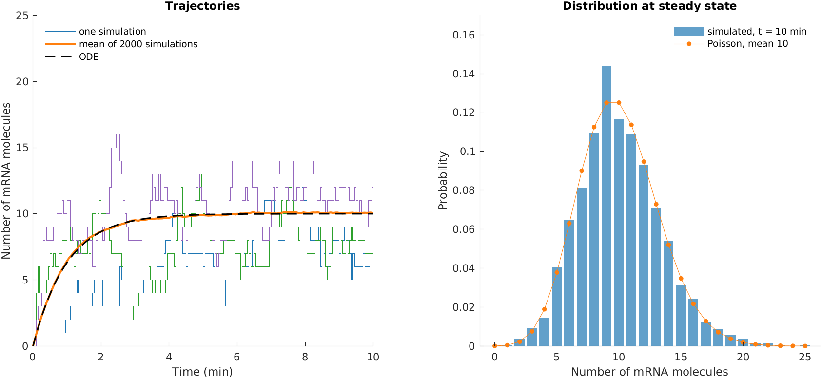

Python

Needs SciPy (for the Poisson distribution).

"""Stochastic production and degradation of an mRNA.

    0 -> M     at rate k          (transcription)
    M -> 0     at rate gamma * M  (degradation)

The deterministic (ODE) model, dM/dt = k - gamma*M, predicts a smooth
rise to M = k/gamma. With few molecules, each reaction is a random
event, simulated here with Gillespie's algorithm. At steady state the
number of molecules follows a Poisson distribution with mean k/gamma.
"""
import numpy as np
from scipy.stats import poisson
import matplotlib.pyplot as plt
import sbp
from sbp.ssa import gillespie

k, gamma = 10.0, 1.0              # per minute
t_grid = np.linspace(0, 10, 201)  # minutes
n_runs = 2000
rng = np.random.default_rng(1)

changes = [[+1], [-1]]


def propensities(x):
    return np.array([k, gamma * x[0]])


runs = np.array([gillespie([0], changes, propensities, t_grid, rng)[:, 0]
                 for _ in range(n_runs)])
final = runs[:, -1]
ode = k / gamma * (1 - np.exp(-gamma * t_grid))

print(f"At t = {t_grid[-1]:g} min, over {n_runs} runs: mean {final.mean():.3f}"
      f", variance {final.var():.3f} (Poisson: both {k / gamma:g})")

# --- Plot
sbp.style()
fig, (ax1, ax2) = plt.subplots(1, 2, figsize=(10, 4))
colors = ["#1f77b4", "#2ca02c", "#9467bd"]
for r, col in zip(range(3), colors):
    ax1.step(t_grid, runs[r], where="post", color=col, lw=1,
             label="one simulation" if r == 0 else None)
ax1.plot(t_grid, runs.mean(axis=0), "-", color="#ff7f0e", lw=2,
         label=f"mean of {n_runs} simulations")
ax1.plot(t_grid, ode, "k--", lw=1.5, label="ODE")
ax1.set_xlabel("Time (min)")
ax1.set_ylabel("Number of mRNA molecules")
ax1.set_ylim(0, 25)
ax1.legend(frameon=False, loc="upper left")
ax1.set_title("Trajectories")

m = np.arange(0, 26)
counts = np.bincount(final.astype(int), minlength=26)[:26] / n_runs
ax2.bar(m, counts, color="#1f77b4", alpha=0.7,
        label=f"simulated, t = {t_grid[-1]:g} min")
ax2.plot(m, poisson.pmf(m, k / gamma), "o-", color="#ff7f0e", ms=4,
         label=f"Poisson, mean {k / gamma:g}")
ax2.set_xlabel("Number of mRNA molecules")
ax2.set_ylabel("Probability")
ax2.set_ylim(0, 0.17)
ax2.legend(frameon=False, loc="upper right")
ax2.set_title("Distribution at steady state")
sbp.save_figure(fig, __file__, "fig-birth-death")

sbp.save_results(__file__, {
    "steady_state": {"mean": final.mean(), "variance": final.var()},
    "mean_trajectory": runs.mean(axis=0)[::20],
})
sbp.show()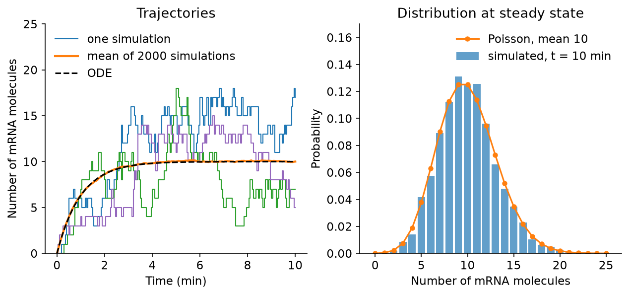

Individual runs (left) are jagged and differ from one another; at steady state, any one of them may hold anywhere from about 3 to 18 molecules. Their average, on the other hand, follows the ODE closely. For reactions such as these, where every propensity is at most linear in the numbers of molecules, the ODE gives the mean behaviour exactly; for nonlinear reactions, such as dimerisation, it is only an approximation. The distribution across runs (right) matches the Poisson distribution.

A useful way to describe the size of fluctuations is the Fano factor, the variance divided by the mean. It is 1 for a Poisson distribution, whatever the mean. Relative fluctuations, measured by the coefficient of variation \(\sigma/\mu = 1/\sqrt{\mu}\), shrink as numbers grow: with 10 molecules they are about 32%, with 10,000 about 1%. That is why ODEs work well for abundant molecules and stochastic models matter for scarce ones.

6.3 Noise in gene expression

Proteins are made from mRNAs, and each mRNA is translated many times before it is degraded. Adding these two steps,

\[ \emptyset \xrightarrow{k_m} \text{M}, \qquad \text{M} \xrightarrow{\gamma_m M} \emptyset, \qquad \text{M} \xrightarrow{k_p M} \text{M} + \text{P}, \qquad \text{P} \xrightarrow{\gamma_p P} \emptyset , \]

the mean number of proteins at steady state is \(k_m k_p / \gamma_m \gamma_p\), and the Fano factor of the protein is approximately \(1 + k_p/(\gamma_m + \gamma_p)\) (Thattai and Oudenaarden 2001). The ratio \(k_p/\gamma_m\) is the mean number of proteins made from one mRNA, the burst size. So two genes can make the same average amount of protein with very different noise: gene A is transcribed often, with small bursts of 2.5 proteins per mRNA, while gene B is transcribed ten times less often, with bursts of 25. Here we simulate each gene for 40,000 minutes and sample the protein number once a minute.

MATLAB

Core MATLAB only.

%% Noise in gene expression: transcription and translation
%     0 -> M       at rate km           (transcription)
%     M -> 0       at rate gm * M       (mRNA degradation)
%     M -> M + P   at rate kp * M       (translation)
%     P -> 0       at rate gp * P       (protein degradation)
% Two genes make the same mean number of proteins, 50. Gene A is
% transcribed often and each mRNA is translated a few times; gene B is
% transcribed rarely and each mRNA is translated many times, so its
% proteins are made in bursts. Theory (for example, Thattai and van
% Oudenaarden, 2001) gives, at steady state,
%     mean P = km*kp/(gm*gp),   Fano factor = var/mean = 1 + kp/(gm + gp).
% Requires: core MATLAB only.

gm = 1.0; gp = 0.1;                     % per minute
names = {'A', 'B'};
km = [2.0 0.2];                         % B: rare transcription,
kp = [2.5 25.0];                        %    big bursts
t_grid = 0:40000;                       % one long run, sampled each minute
burn_in = 200;                          % discard the approach to steady state
rng(1);

% Changes in (M, P) for each of the four reactions
changes = [1 0; -1 0; 0 1; 0 -1];

traces = zeros(numel(t_grid), 2);
for g = 1:2
    propensities = @(x) [km(g), gm * x(1), kp(g) * x(1), gp * x(2)];
    X = sbp.gillespie([0 0], changes, propensities, t_grid);
    traces(:, g) = X(:, 2);
    P = X(burn_in + 1:end, 2);
    results.(names{g}) = struct('mean', mean(P), ...
        'fano', var(P, 1) / mean(P));
    fprintf(['Gene %s: mean %.1f (theory %g), Fano factor %.2f ' ...
        '(theory %.2f)\n'], names{g}, mean(P), km(g) * kp(g) / (gm * gp), ...
        var(P, 1) / mean(P), 1 + kp(g) / (gm + gp));
end

%% Plot
colors = [0.122 0.467 0.706; 1.000 0.498 0.055];
fig = figure('Position', [100 100 1000 400]);
subplot(1, 3, [1 2])
window = 1001:1301;
for g = 1:2
    plot(t_grid(window) - t_grid(window(1)), traces(window, g), ...
        'Color', colors(g, :), 'LineWidth', 1.2);
    hold on
end
xlabel('Time (min)'); ylabel('Number of protein molecules');
title('Same mean, different noise');
legend({'gene A', 'gene B'}, 'Location', 'northwest', 'Box', 'off');
box off

subplot(1, 3, 3)
edges = 0:5:250;
for g = 1:2
    h = histcounts(traces(burn_in + 1:end, g), edges, ...
        'Normalization', 'pdf');
    stairs(edges, [h h(end)], 'Color', colors(g, :), 'LineWidth', 1.5);
    hold on
end
xlabel('Number of protein molecules'); ylabel('Probability density');
title('Distribution');
legend({'gene A', 'gene B'}, 'Box', 'off');
box off
sbp.save_figure(fig, mfilename('fullpath'), 'fig-gene-expression');

sbp.save_results(mfilename('fullpath'), results);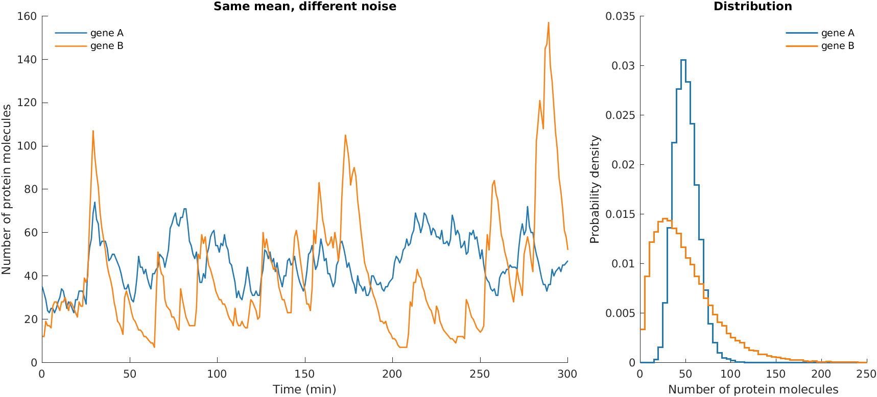

Python

Needs NumPy and Matplotlib.

"""Noise in gene expression: transcription and translation.

    0 -> M       at rate km           (transcription)
    M -> 0       at rate gm * M       (mRNA degradation)
    M -> M + P   at rate kp * M       (translation)
    P -> 0       at rate gp * P       (protein degradation)

Two genes make the same mean number of proteins, 50. Gene A is
transcribed often and each mRNA is translated a few times; gene B is
transcribed rarely and each mRNA is translated many times, so its
proteins are made in bursts. Theory (for example, Thattai and van
Oudenaarden, 2001) gives, at steady state,
    mean P = km*kp/(gm*gp),   Fano factor = var/mean = 1 + kp/(gm + gp).
"""
import numpy as np
import matplotlib.pyplot as plt
import sbp
from sbp.ssa import gillespie

gm, gp = 1.0, 0.1                       # per minute
genes = {"A": {"km": 2.0, "kp": 2.5},   # frequent transcription
         "B": {"km": 0.2, "kp": 25.0}}  # rare transcription, big bursts
t_grid = np.arange(0, 40001.0)          # one long run, sampled each minute
burn_in = 200                           # discard the approach to steady state
rng = np.random.default_rng(1)

# Changes in (M, P) for each of the four reactions
changes = [[1, 0], [-1, 0], [0, 1], [0, -1]]

results = {}
traces = {}
for name, g in genes.items():
    def propensities(x, km=g["km"], kp=g["kp"]):
        M, P = x
        return np.array([km, gm * M, kp * M, gp * P])

    X = gillespie([0, 0], changes, propensities, t_grid, rng)
    P = X[burn_in:, 1]
    theory_mean = g["km"] * g["kp"] / (gm * gp)
    theory_fano = 1 + g["kp"] / (gm + gp)
    results[name] = {"mean": P.mean(), "fano": P.var() / P.mean()}
    traces[name] = X[:, 1]
    print(f"Gene {name}: mean {P.mean():.1f} (theory {theory_mean:g}), "
          f"Fano factor {P.var() / P.mean():.2f} (theory {theory_fano:.2f})")

# --- Plot
sbp.style()
fig, (ax1, ax2) = plt.subplots(1, 2, figsize=(10, 4),
                               gridspec_kw={"width_ratios": [2, 1]})
window = slice(1000, 1301)
colors = {"A": "#1f77b4", "B": "#ff7f0e"}
for name in genes:
    ax1.plot(t_grid[window] - t_grid[window][0], traces[name][window],
             color=colors[name], lw=1.2, label=f"gene {name}")
    ax2.hist(traces[name][burn_in:], bins=np.arange(0, 251, 5),
             density=True, histtype="step", lw=1.5, color=colors[name],
             label=f"gene {name}")
ax1.set_xlabel("Time (min)")
ax1.set_ylabel("Number of protein molecules")
ax1.set_title("Same mean, different noise")
ax1.legend(frameon=False, loc="upper left")
ax2.set_xlabel("Number of protein molecules")
ax2.set_ylabel("Probability density")
ax2.set_title("Distribution")
ax2.legend(frameon=False)
sbp.save_figure(fig, __file__, "fig-gene-expression")

sbp.save_results(__file__, results)
sbp.show()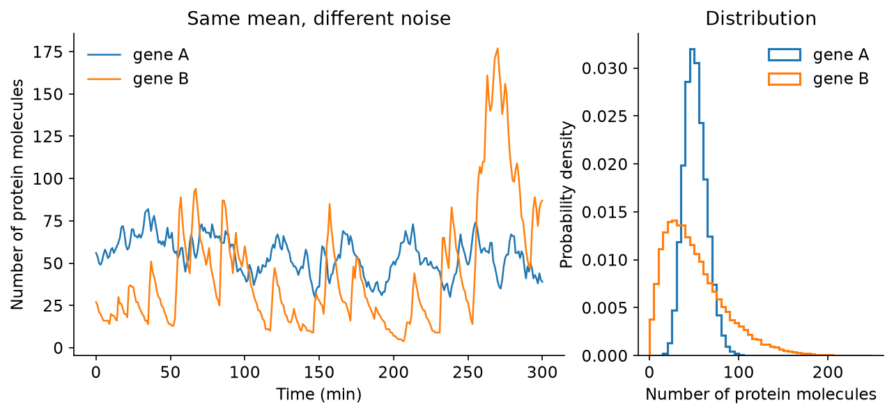

Both genes average about 50 proteins, but gene B jumps up in bursts, each time one of its rare mRNAs is translated many times over, and then decays; its Fano factor is about 24, against about 3 for gene A, and its distribution is wide and skewed. Ozbudak and colleagues found exactly this in Bacillus subtilis: increasing translation increased noise far more than increasing transcription did (Ozbudak et al. 2002). Cells can therefore tune their noise, and not just their mean expression, through the balance of transcription and translation.

Since MATLAB and Python draw different random numbers, the two versions give slightly different estimates. The automated checks require both to be within 10% of theory for the mRNA example, and within 15% for the noisier protein estimates.

6.4 Exercises

1. In the mRNA example, start each run with 50 molecules in place of none. How does the mean approach the steady state? Compare with the solution of the ODE.
2. Add a dimerisation reaction, \(2\text{P} \to \text{D}\), with propensity \(k_d P(P-1)/2\), to the birth–death model for a protein P. Compare the mean of many SSA runs with the solution of the corresponding ODE for small and large numbers of molecules. When do they differ?
3. For the gene-expression model, vary \(k_p\) from 1 to 50 while adjusting \(k_m\) to keep the mean at 50 proteins. Plot the Fano factor against the burst size \(k_p/\gamma_m\) and compare with the theory.
4. Simulating every reaction becomes slow when molecules are abundant. Look up the tau-leaping method, which fires many reactions in each time step, and implement it for the mRNA example. How large can the time step be before the distribution is visibly wrong?

6.5 Going further

Noise is not always a nuisance. In circuits with two stable states, such as the toggle switch, noise can flip cells between states, letting a population hedge its bets. Exploring such circuits needs both the ODE tools of Chapter 3 and the stochastic tools of this chapter.

Gillespie, Daniel T. 1977. “Exact Stochastic Simulation of Coupled Chemical Reactions.” The Journal of Physical Chemistry 81 (25): 2340–61. https://doi.org/10.1021/j100540a008.

Gillespie, Daniel T. 2007. “Stochastic Simulation of Chemical Kinetics.” Annual Review of Physical Chemistry 58: 35–55. https://doi.org/10.1146/annurev.physchem.58.032806.104637.

Ozbudak, Ertugrul M., Mukund Thattai, Iren Kurtser, Alan D. Grossman, and Alexander van Oudenaarden. 2002. “Regulation of Noise in the Expression of a Single Gene.” Nature Genetics 31 (1): 69–73. https://doi.org/10.1038/ng869.

Raj, Arjun, and Alexander van Oudenaarden. 2008. “Nature, Nurture, or Chance: Stochastic Gene Expression and Its Consequences.” Cell 135 (2): 216–26. https://doi.org/10.1016/j.cell.2008.09.050.

Thattai, Mukund, and Alexander van Oudenaarden. 2001. “Intrinsic Noise in Gene Regulatory Networks.” Proceedings of the National Academy of Sciences 98 (15): 8614–19. https://doi.org/10.1073/pnas.151588598.