7  Constraint-based modelling

Kinetic models need rate laws and parameters that are rarely known for more than a handful of reactions. Constraint-based modelling sidesteps this. It asks only for the stoichiometry of a metabolic network, and a few bounds on the fluxes, and then asks: of all the flux distributions the network can support at steady state, which ones are possible, and which one is best for a given objective, such as growth?

This chapter works through flux balance analysis (FBA) and flux variability analysis (FVA), first on a small toy network that you can check by hand, and then on a real metabolic model of E. coli.

NoteIn the book

Chapter 8, Introduction to Constraint-Based Modelling: the stoichiometric matrix (§8.2), steady-state mass balance (§8.3), objective functions (§8.4), FBA as a linear program (§8.5), the worked toy example (§8.6), FVA (§8.7) and practical issues such as multiple optima and ATP maintenance (§8.8).

7.1 The toy network

We use the small network of the book’s Fig. 8.1: eight metabolites, seven internal reactions, two exchange reactions that connect the cell to its surroundings, and a “biomass” reaction that drains the building blocks the cell needs to grow.

Table 7.1: The toy network. Fluxes are in mmol/gDW/h.

Reaction	Equation	Flux	Bounds
R1	A → ATP + B	\(v_1\)	[0, 1000]
R2	A → C	\(v_2\)	[0, 1000]
R3	C → ATP + B	\(v_3\)	[0, 1000]
R4	B \(\rightleftharpoons\) 2 D	\(v_4\)	[−1000, 1000]
R5	B → F	\(v_5\)	[0, 1000]
R6	D \(\rightleftharpoons\) E	\(v_6\)	[−1000, 1000]
R7	D + ATP → G	\(v_7\)	[0, 1000]
E1	→ A	\(b_1\)	[0, 1000]
E2	E \(\rightleftharpoons\)	\(b_2\)	[−1000, 1000]
Biomass	F + 2 G + 10 ATP →	\(v_\text{bio}\)	[0, 1000]

Each reaction becomes a column of the stoichiometric matrix \(\mathbf{S}\), with one row per metabolite: negative entries for what a reaction consumes and positive entries for what it produces. At steady state, every metabolite is produced exactly as fast as it is consumed, so any feasible flux vector \(\mathbf{v}\) satisfies

\[ \mathbf{S}\mathbf{v} = \mathbf{0}. \]

With eight equations and ten unknowns, this system has infinitely many solutions. FBA picks one by optimising an objective, here the biomass flux.

7.2 Flux balance analysis

FBA is a linear program (LP):

\[ \max_{\mathbf{v}}\ \mathbf{c}^\top\mathbf{v} \quad\text{subject to}\quad \mathbf{S}\mathbf{v} = \mathbf{0},\qquad \mathbf{v}_\text{lb} \le \mathbf{v} \le \mathbf{v}_\text{ub}, \]

where \(\mathbf{c}\) picks out the objective; it has a 1 in the position of \(v_\text{bio}\) and zeros elsewhere. Any LP solver will do. Both linprog functions minimise, so we minimise \(-\mathbf{c}^\top\mathbf{v}\) instead.

MATLAB

Needs the Optimization Toolbox (for linprog).

%% Flux balance analysis of a toy metabolic network
% The network is the one in Fig. 8.1 / Table 8.2 of the book: 8 metabolites,
% 7 internal reactions, 2 exchange reactions and a 'biomass' reaction.
% FBA is solved directly as a linear program with linprog.
% Requires: Optimization Toolbox (for linprog).

%% The network
rxns = {'v1', 'v2', 'v3', 'v4', 'v5', 'v6', 'v7', 'b1', 'b2', 'vbio'};
mets = {'A', 'B', 'C', 'D', 'E', 'F', 'G', 'ATP'};

% Stoichiometric matrix: one row per metabolite, one column per reaction
%    v1  v2  v3  v4  v5  v6  v7  b1  b2 vbio
S = [-1  -1   0   0   0   0   0   1   0   0     % A
      1   0   1  -1  -1   0   0   0   0   0     % B
      0   1  -1   0   0   0   0   0   0   0     % C
      0   0   0   2   0  -1  -1   0   0   0     % D
      0   0   0   0   0   1   0   0  -1   0     % E
      0   0   0   0   1   0   0   0   0  -1     % F
      0   0   0   0   0   0   1   0   0  -2     % G
      1   0   1   0   0   0  -1   0   0 -10];   % ATP

% Bounds (mmol/gDW/h): reversible reactions v4, v6 and b2 may run backwards
lb = [0 0 0 -1000 0 -1000 0 0 -1000 0]';
ub = 1000 * ones(numel(rxns), 1);

% Objective: maximise the biomass flux vbio
c = zeros(numel(rxns), 1);
c(strcmp(rxns, 'vbio')) = 1;

%% Solve: max c'v  s.t.  Sv = 0,  lb <= v <= ub
% linprog minimises, so we minimise -c'v
opts = optimoptions('linprog', 'Display', 'none');
beq = zeros(numel(mets), 1);
[v, fval, exitflag] = linprog(-c, [], [], S, beq, lb, ub, opts);
growth = -fval;

fprintf('Exit flag: %d (1 means optimal)\n', exitflag);
fprintf('Maximum biomass flux vbio = %g\n', growth);
for k = 1:numel(rxns)
    fprintf('  %4s = %8.1f\n', rxns{k}, v(k));
end
fprintf('Largest mass-balance violation |Sv| = %.1e\n', max(abs(S*v)));

%% Plot the flux distribution
fig = figure;
bar(categorical(rxns, rxns), v, 'FaceColor', [0.122 0.467 0.706]);
xlabel('Reaction');
ylabel('Flux (mmol/gDW/h)');
title(sprintf('An optimal flux distribution (vbio = %g)', growth));
box off
sbp.save_figure(fig, mfilename('fullpath'), 'fig-toy-fba');

results.growth = growth;
results.fluxes = cell2struct(num2cell(v), rxns, 1);
results.max_mass_balance_error = max(abs(S*v));
sbp.save_results(mfilename('fullpath'), results);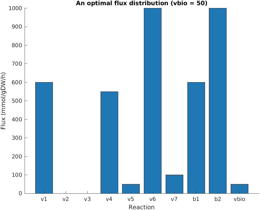

Python

Needs SciPy (for linprog).

"""Flux balance analysis of a toy metabolic network.

The network is the one in Fig. 8.1 / Table 8.2 of the book: 8 metabolites,
7 internal reactions, 2 exchange reactions and a 'biomass' reaction.
FBA is solved directly as a linear program with SciPy.
"""
import numpy as np
from scipy.optimize import linprog
import matplotlib.pyplot as plt
import sbp

# --- The network
rxns = ["v1", "v2", "v3", "v4", "v5", "v6", "v7", "b1", "b2", "vbio"]
mets = ["A", "B", "C", "D", "E", "F", "G", "ATP"]

# Stoichiometric matrix: one row per metabolite, one column per reaction
#             v1  v2  v3  v4  v5  v6  v7  b1  b2 vbio
S = np.array([[-1, -1,  0,  0,  0,  0,  0,  1,  0,   0],   # A
              [ 1,  0,  1, -1, -1,  0,  0,  0,  0,   0],   # B
              [ 0,  1, -1,  0,  0,  0,  0,  0,  0,   0],   # C
              [ 0,  0,  0,  2,  0, -1, -1,  0,  0,   0],   # D
              [ 0,  0,  0,  0,  0,  1,  0,  0, -1,   0],   # E
              [ 0,  0,  0,  0,  1,  0,  0,  0,  0,  -1],   # F
              [ 0,  0,  0,  0,  0,  0,  1,  0,  0,  -2],   # G
              [ 1,  0,  1,  0,  0,  0, -1,  0,  0, -10]])  # ATP

# Bounds (mmol/gDW/h): reversible reactions v4, v6 and b2 may run backwards
lb = np.array([0, 0, 0, -1000, 0, -1000, 0, 0, -1000, 0])
ub = np.full(len(rxns), 1000)

# Objective: maximise the biomass flux vbio
c = np.zeros(len(rxns))
c[rxns.index("vbio")] = 1

# --- Solve: max c'v  s.t.  Sv = 0,  lb <= v <= ub
# linprog minimises, so we minimise -c'v
res = linprog(-c, A_eq=S, b_eq=np.zeros(len(mets)),
              bounds=list(zip(lb, ub)), method="highs")
v = res.x + 0.0  # (+ 0.0 turns any -0.0 into 0.0 for printing)
growth = -res.fun

print(f"Status: {res.message}")
print(f"Maximum biomass flux vbio = {growth:g}")
for r, flux in zip(rxns, v):
    print(f"  {r:>4s} = {flux:8.1f}")
print(f"Largest mass-balance violation |Sv| = {np.abs(S @ v).max():.1e}")

# --- Plot the flux distribution
sbp.style()
fig, ax = plt.subplots()
ax.bar(rxns, v, color="#1f77b4")
ax.set_xlabel("Reaction")
ax.set_ylabel("Flux (mmol/gDW/h)")
ax.set_title(f"An optimal flux distribution (vbio = {growth:g})")
sbp.save_figure(fig, __file__, "fig-toy-fba")

sbp.save_results(__file__, {
    "growth": growth,
    "fluxes": dict(zip(rxns, v)),
    "max_mass_balance_error": np.abs(S @ v).max(),
})
sbp.show()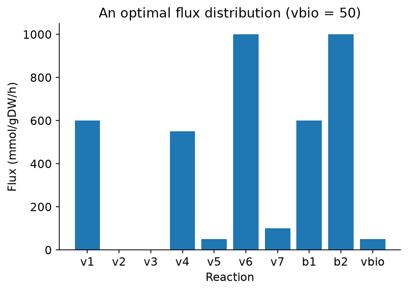

The maximum biomass flux is \(v_\text{bio} = 50\), the same as in the book (Eq. 8.8). What limits it? Follow the stoichiometry: every unit of biomass needs 2 G, and so 2 units of flux through R7, and 10 ATP. Balancing ATP, B and D in turn shows that \(v_4 = 11\,v_\text{bio}\) and \(v_6 = 20\,v_\text{bio}\), so the upper bound of 1000 on \(v_6\) (and on \(b_2\), which must equal \(v_6\)) caps growth at 50.

NoteThe optimal growth rate is unique; the flux distribution is not

R1 and the route R2 → R3 both turn A into ATP + B, so the cell can split the 600 units of A between them in any proportion and grow equally well. The book shows two such solutions (Eqs. 8.8 and 8.9). Which one you get depends on the solver, and the MATLAB and Python versions above may print different values of \(v_1\), \(v_2\) and \(v_3\). Both are correct. This is why our automated checks compare only the growth rate for this example, and why the next section matters.

7.3 Flux variability analysis

FVA maps out all the optimal (or near-optimal) solutions at once. First solve the FBA problem to get the optimal objective \(f^*\). Then, for each reaction \(j\) in turn, find the smallest and the largest flux it can carry while growth stays at least a fraction \(\alpha\) of the optimum:

\[ \min_{\mathbf{v}} / \max_{\mathbf{v}}\ v_j \quad\text{subject to}\quad \mathbf{S}\mathbf{v} = \mathbf{0},\quad \mathbf{v}_\text{lb} \le \mathbf{v} \le \mathbf{v}_\text{ub},\quad \mathbf{c}^\top\mathbf{v} \ge \alpha f^*. \]

That is two LPs per reaction. The code below runs FVA at \(\alpha = 1\) (exactly optimal growth) and \(\alpha = 0.9\).

MATLAB

Needs the Optimization Toolbox (for linprog).

%% Flux variability analysis (FVA) of the toy metabolic network
% FBA gives one optimal flux distribution, but often many exist. FVA finds,
% for every reaction, the smallest and largest flux compatible with
% (a chosen fraction of) the optimal growth rate.
% Requires: Optimization Toolbox (for linprog).

%% The network (same as toy_fba.m; book Fig. 8.1)
rxns = {'v1', 'v2', 'v3', 'v4', 'v5', 'v6', 'v7', 'b1', 'b2', 'vbio'};
%    v1  v2  v3  v4  v5  v6  v7  b1  b2 vbio
S = [-1  -1   0   0   0   0   0   1   0   0     % A
      1   0   1  -1  -1   0   0   0   0   0     % B
      0   1  -1   0   0   0   0   0   0   0     % C
      0   0   0   2   0  -1  -1   0   0   0     % D
      0   0   0   0   0   1   0   0  -1   0     % E
      0   0   0   0   1   0   0   0   0  -1     % F
      0   0   0   0   0   0   1   0   0  -2     % G
      1   0   1   0   0   0  -1   0   0 -10];   % ATP
lb = [0 0 0 -1000 0 -1000 0 0 -1000 0]';
ub = 1000 * ones(numel(rxns), 1);
n = numel(rxns);
c = zeros(n, 1);
c(strcmp(rxns, 'vbio')) = 1;
opts = optimoptions('linprog', 'Display', 'none');

%% Step 1: FBA, to find the optimal growth rate f*
[~, fval] = linprog(-c, [], [], S, zeros(size(S, 1), 1), lb, ub, opts);
f_star = -fval;

%% Step 2: FVA at 100% and at 90% of the optimum
[vmin100, vmax100] = fva(S, lb, ub, c, 1.0 * f_star, opts);
[vmin90,  vmax90]  = fva(S, lb, ub, c, 0.9 * f_star, opts);

fprintf('Optimal growth f* = %g\n', f_star);
fprintf('%5s %8s %8s   (at 100%% of f*)\n', 'rxn', 'min', 'max');
for j = 1:n
    fprintf('%5s %8.1f %8.1f\n', rxns{j}, vmin100(j), vmax100(j));
end

%% Plot: flux ranges at 100% and 90% of optimal growth
blue = [0.122 0.467 0.706];
orange = [1.000 0.498 0.055];
fig = figure;
hold on
y = 1:n;
for j = 1:n
    plot([vmin90(j) vmax90(j)], y(j) + [0.15 0.15], '-|', 'Color', orange, ...
        'LineWidth', 6, 'MarkerSize', 10);
    plot([vmin100(j) vmax100(j)], y(j) - [0.15 0.15], '-|', 'Color', blue, ...
        'LineWidth', 6, 'MarkerSize', 10);
end
set(gca, 'YTick', y, 'YTickLabel', rxns, 'YDir', 'reverse');
xlabel('Flux (mmol/gDW/h)');
title('Flux variability analysis');
h = [plot(NaN, NaN, '-', 'Color', orange, 'LineWidth', 6), ...
     plot(NaN, NaN, '-', 'Color', blue, 'LineWidth', 6)];
legend(h, {'90% of optimum', '100% of optimum'}, ...
    'Location', 'northeast', 'Box', 'off');
box off
sbp.save_figure(fig, mfilename('fullpath'), 'fig-toy-fva');

results.growth = f_star;
results.fva100.min = cell2struct(num2cell(vmin100), rxns, 1);
results.fva100.max = cell2struct(num2cell(vmax100), rxns, 1);
results.fva90.min = cell2struct(num2cell(vmin90), rxns, 1);
results.fva90.max = cell2struct(num2cell(vmax90), rxns, 1);
sbp.save_results(mfilename('fullpath'), results);

%% Local function
function [vmin, vmax] = fva(S, lb, ub, c, f_min, opts)
% Min and max of every flux, subject to growth c'v >= f_min.
% The extra constraint is written as -c'v <= -f_min.
n = numel(lb);
vmin = zeros(n, 1);
vmax = zeros(n, 1);
beq = zeros(size(S, 1), 1);
for j = 1:n
    e = zeros(n, 1);
    e(j) = 1;
    [~, vmin(j)] = linprog(e, -c', -f_min, S, beq, lb, ub, opts);
    [~, fmax] = linprog(-e, -c', -f_min, S, beq, lb, ub, opts);
    vmax(j) = -fmax;
end
end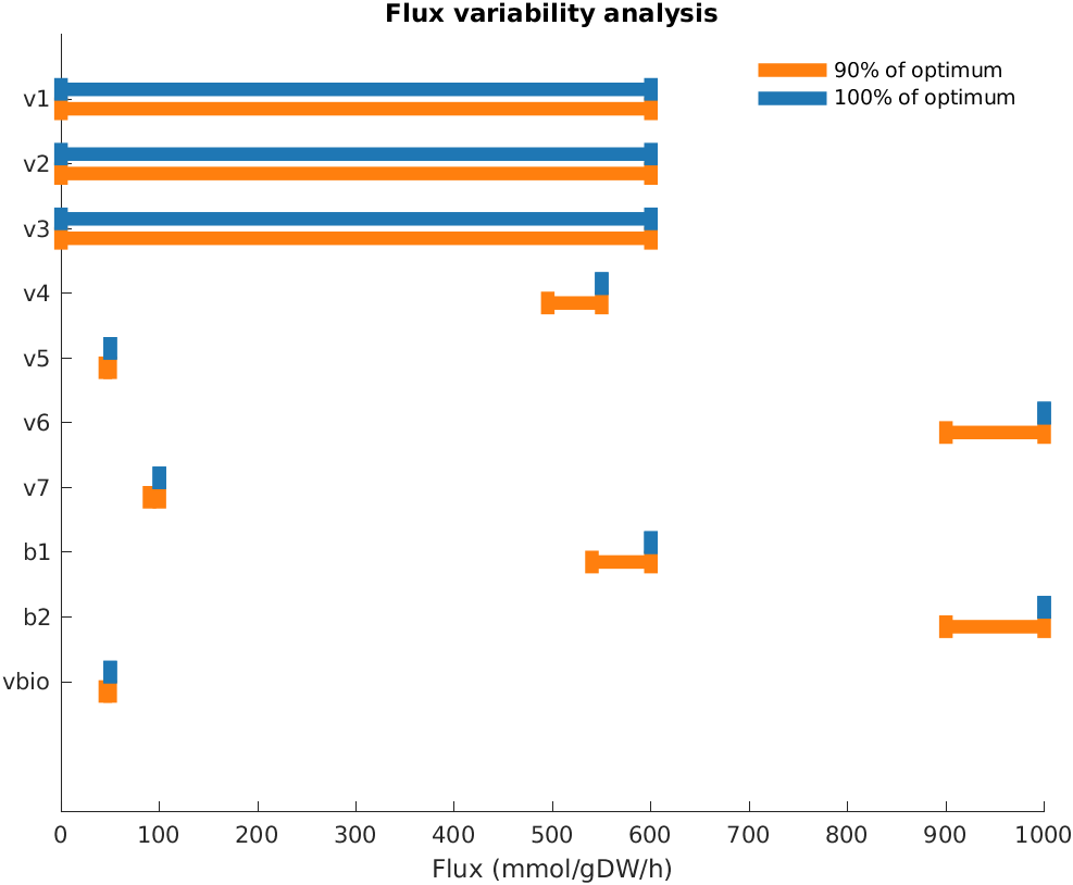

Python

Needs SciPy (for linprog).

"""Flux variability analysis (FVA) of the toy metabolic network.

FBA gives one optimal flux distribution, but often many exist. FVA finds,
for every reaction, the smallest and largest flux compatible with
(a chosen fraction of) the optimal growth rate.
"""
import numpy as np
from scipy.optimize import linprog
import matplotlib.pyplot as plt
import sbp

# --- The network (same as toy_fba.py; book Fig. 8.1)
rxns = ["v1", "v2", "v3", "v4", "v5", "v6", "v7", "b1", "b2", "vbio"]
#             v1  v2  v3  v4  v5  v6  v7  b1  b2 vbio
S = np.array([[-1, -1,  0,  0,  0,  0,  0,  1,  0,   0],   # A
              [ 1,  0,  1, -1, -1,  0,  0,  0,  0,   0],   # B
              [ 0,  1, -1,  0,  0,  0,  0,  0,  0,   0],   # C
              [ 0,  0,  0,  2,  0, -1, -1,  0,  0,   0],   # D
              [ 0,  0,  0,  0,  0,  1,  0,  0, -1,   0],   # E
              [ 0,  0,  0,  0,  1,  0,  0,  0,  0,  -1],   # F
              [ 0,  0,  0,  0,  0,  0,  1,  0,  0,  -2],   # G
              [ 1,  0,  1,  0,  0,  0, -1,  0,  0, -10]])  # ATP
lb = np.array([0, 0, 0, -1000, 0, -1000, 0, 0, -1000, 0])
ub = np.full(len(rxns), 1000)
bounds = list(zip(lb, ub))
n = len(rxns)
c = np.zeros(n)
c[rxns.index("vbio")] = 1
zeros = np.zeros(S.shape[0])

# --- Step 1: FBA, to find the optimal growth rate f*
fba = linprog(-c, A_eq=S, b_eq=zeros, bounds=bounds, method="highs")
f_star = -fba.fun


def fva(fraction):
    """Min and max of every flux, subject to growth >= fraction * f*."""
    # The extra constraint c'v >= fraction*f*, written as -c'v <= -fraction*f*
    A_ub, b_ub = -c[np.newaxis, :], [-fraction * f_star]
    vmin, vmax = np.zeros(n), np.zeros(n)
    for j in range(n):
        e = np.zeros(n)
        e[j] = 1
        vmin[j] = linprog(e, A_ub=A_ub, b_ub=b_ub, A_eq=S, b_eq=zeros,
                          bounds=bounds, method="highs").fun
        vmax[j] = -linprog(-e, A_ub=A_ub, b_ub=b_ub, A_eq=S, b_eq=zeros,
                           bounds=bounds, method="highs").fun
    return vmin, vmax


# --- Step 2: FVA at 100% and at 90% of the optimum
vmin100, vmax100 = fva(1.0)
vmin90, vmax90 = fva(0.9)

print(f"Optimal growth f* = {f_star:g}")
print(f"{'rxn':>5s} {'min':>8s} {'max':>8s}   (at 100% of f*)")
for r, lo, hi in zip(rxns, vmin100, vmax100):
    print(f"{r:>5s} {lo:8.1f} {hi:8.1f}")

# --- Plot: flux ranges at 100% and 90% of optimal growth
sbp.style()
fig, ax = plt.subplots()
y = np.arange(n)
ax.hlines(y + 0.15, vmin90, vmax90, color="#ff7f0e", lw=6,
          label="90% of optimum")
ax.hlines(y - 0.15, vmin100, vmax100, color="#1f77b4", lw=6,
          label="100% of optimum")
# Fixed fluxes have zero width, so mark both ends
ax.plot(vmin100, y - 0.15, "|", color="#1f77b4", ms=10)
ax.plot(vmin90, y + 0.15, "|", color="#ff7f0e", ms=10)
ax.set_yticks(y, rxns)
ax.invert_yaxis()
ax.set_xlabel("Flux (mmol/gDW/h)")
ax.set_title("Flux variability analysis")
ax.legend(loc="upper right", frameon=False)
sbp.save_figure(fig, __file__, "fig-toy-fva")

sbp.save_results(__file__, {
    "growth": f_star,
    "fva100": {"min": dict(zip(rxns, vmin100)),
               "max": dict(zip(rxns, vmax100))},
    "fva90": {"min": dict(zip(rxns, vmin90)),
              "max": dict(zip(rxns, vmax90))},
})
sbp.show()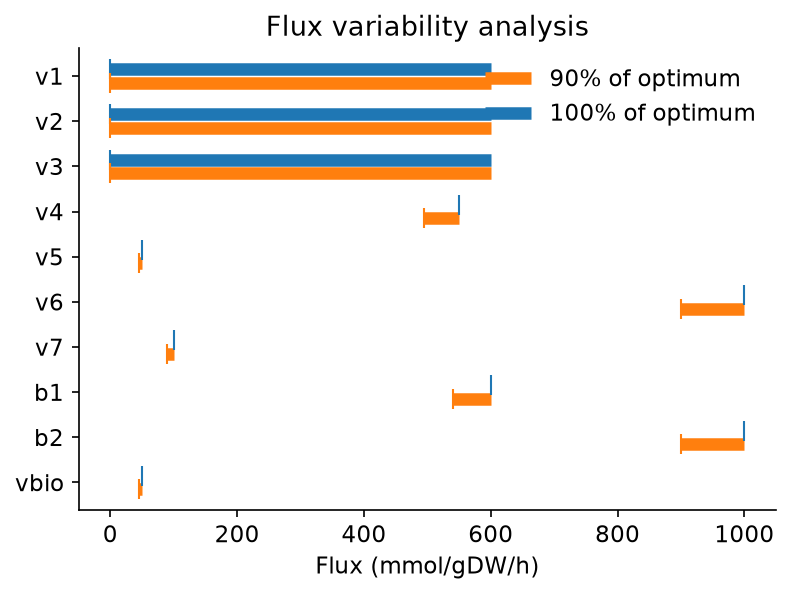

At optimal growth, \(v_1\), \(v_2\) and \(v_3\) can each take any value between 0 and 600, while every other flux is fixed. These are exactly the ranges in the book (Eq. 8.12). Relaxing growth to 90% of the optimum widens the other ranges too, because the reactions that limit growth no longer have to run at their maximum.

7.4 A genome-scale example: E. coli core

The same ideas carry over unchanged to real networks. The E. coli core model (Orth et al. 2010) has 95 reactions, 72 metabolites and 137 genes, covering glycolysis, the pentose phosphate pathway, the TCA cycle and oxidative phosphorylation. At this scale we no longer write \(\mathbf{S}\) by hand. A standard model file (SBML) is read by a modelling package, COBRApy in Python and the COBRA Toolbox in MATLAB, which builds and solves the LP for us.

Two things to know when reading the code:

• Exchange reactions such as EX_glc__D_e (glucose) and EX_o2_e (oxygen) are written as secretion, so uptake is a negative flux. Allowing up to 10 mmol/gDW/h of glucose uptake therefore means setting the lower bound to −10.
• The model includes an ATP maintenance reaction, ATPM, with a lower bound of 8.39 mmol/gDW/h: ATP the cell must spend just to stay alive, whether it grows or not.

MATLAB

Needs the COBRA Toolbox; run initCobraToolbox once per session before this script.

%% FBA on the E. coli core metabolic model with the COBRA Toolbox
% 1. Predict growth with and without oxygen.
% 2. Vary the glucose uptake rate and watch growth respond.
% Requires: COBRA Toolbox (run initCobraToolbox once per session first).

% The .mat file is the same model as the SBML file the Python version reads
% (made by tools/make_mat_model.py); reading SBML in MATLAB needs libSBML.
model = readCbModel(fullfile(sbp.data_dir(), 'e_coli_core.mat'));
fprintf('%d reactions, %d metabolites, %d genes\n', ...
    numel(model.rxns), numel(model.mets), numel(model.genes));
fprintf('Objective: %s\n', strjoin(model.rxns(model.c ~= 0), ', '));

%% 1. Aerobic vs anaerobic growth
% Default medium: glucose uptake up to 10 mmol/gDW/h, oxygen unlimited.
% Uptake is a negative flux through an exchange reaction, hence lower bounds.
aerobic = optimizeCbModel(model, 'max');
fprintf('Aerobic growth rate:   %.4f /h\n', aerobic.f);

modelAnaerobic = changeRxnBounds(model, 'EX_o2_e', 0, 'l');  % no oxygen uptake
anaerobic = optimizeCbModel(modelAnaerobic, 'max');
fprintf('Anaerobic growth rate: %.4f /h\n', anaerobic.f);

%% 2. Growth as a function of glucose uptake
uptake = 0:0.5:20;  % mmol/gDW/h
growthAer = growth_curve(model, 1000, uptake);  % O2 effectively unlimited
growthO2_10 = growth_curve(model, 10, uptake);  % O2 uptake at most 10
growthAnaer = growth_curve(model, 0, uptake);   % no O2

%% Plot
fig = figure;
plot(uptake, growthAer, 'o-', 'Color', [0.122 0.467 0.706], 'MarkerSize', 4);
hold on
plot(uptake, growthO2_10, '^-', 'Color', [0.173 0.627 0.173], 'MarkerSize', 4);
plot(uptake, growthAnaer, 's-', 'Color', [1.000 0.498 0.055], 'MarkerSize', 4);
xlabel('Maximum glucose uptake (mmol/gDW/h)');
ylabel('Growth rate (1/h)');
title('E. coli core: growth vs glucose uptake');
legend({'O_2 unlimited', 'O_2 uptake \leq 10', 'no O_2'}, ...
    'Location', 'northwest', 'Box', 'off');
box off
sbp.save_figure(fig, mfilename('fullpath'), 'fig-ecoli-glucose');

results.n_reactions = numel(model.rxns);
results.growth_aerobic = aerobic.f;
results.growth_anaerobic = anaerobic.f;
results.glucose_uptake = uptake;
results.growth_vs_glucose_aerobic = growthAer;
results.growth_vs_glucose_o2_10 = growthO2_10;
results.growth_vs_glucose_anaerobic = growthAnaer;
sbp.save_results(mfilename('fullpath'), results);

%% Local function
function growth = growth_curve(model, o2UptakeLimit, uptake)
% Maximum growth for each glucose uptake limit; NaN where the LP is infeasible.
model = changeRxnBounds(model, 'EX_o2_e', -o2UptakeLimit, 'l');
growth = nan(size(uptake));
for k = 1:numel(uptake)
    m = changeRxnBounds(model, 'EX_glc__D_e', -uptake(k), 'l');
    sol = optimizeCbModel(m, 'max');
    if sol.stat == 1  % 1 means an optimal solution was found
        growth(k) = sol.f;
    end
end
end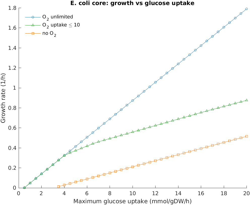

Python

Needs COBRApy.

"""FBA on the E. coli core metabolic model with COBRApy.

1. Predict growth with and without oxygen.
2. Vary the glucose uptake rate and watch growth respond.
"""
import math

import numpy as np
import matplotlib.pyplot as plt
import cobra
import sbp

model = cobra.io.read_sbml_model(str(sbp.DATA / "e_coli_core.xml"))
print(f"{model.id}: {len(model.reactions)} reactions, "
      f"{len(model.metabolites)} metabolites, {len(model.genes)} genes")
objective = cobra.util.solver.linear_reaction_coefficients(model)
print("Objective:", ", ".join(r.id for r in objective))

# --- 1. Aerobic vs anaerobic growth
# Default medium: glucose uptake up to 10 mmol/gDW/h, oxygen unlimited.
# Uptake is a negative flux through an exchange reaction, hence lower bounds.
aerobic = model.optimize()
print(f"Aerobic growth rate:   {aerobic.objective_value:.4f} /h")

with model:  # changes inside 'with' are undone afterwards
    model.reactions.EX_o2_e.lower_bound = 0  # no oxygen uptake
    anaerobic = model.optimize()
print(f"Anaerobic growth rate: {anaerobic.objective_value:.4f} /h")

# --- 2. Growth as a function of glucose uptake
uptake = np.arange(0, 20.5, 0.5)  # mmol/gDW/h


def growth_curve(o2_uptake_limit):
    """Maximum growth for each glucose uptake limit; NaN where infeasible."""
    growth = []
    with model:
        model.reactions.EX_o2_e.lower_bound = -o2_uptake_limit
        for u in uptake:
            model.reactions.EX_glc__D_e.lower_bound = -u
            # slim_optimize returns NaN when the LP is infeasible
            growth.append(model.slim_optimize(error_value=math.nan))
    return np.array(growth)


growth_aer = growth_curve(1000)    # oxygen effectively unlimited
growth_o2_10 = growth_curve(10)    # oxygen uptake at most 10 mmol/gDW/h
growth_anaer = growth_curve(0)     # no oxygen

# --- Plot
sbp.style()
fig, ax = plt.subplots()
ax.plot(uptake, growth_aer, "o-", color="#1f77b4", ms=4,
        label="O$_2$ unlimited")
ax.plot(uptake, growth_o2_10, "^-", color="#2ca02c", ms=4,
        label="O$_2$ uptake ≤ 10")
ax.plot(uptake, growth_anaer, "s-", color="#ff7f0e", ms=4,
        label="no O$_2$")
ax.set_xlabel("Maximum glucose uptake (mmol/gDW/h)")
ax.set_ylabel("Growth rate (1/h)")
ax.set_title("E. coli core: growth vs glucose uptake")
ax.legend(frameon=False)
sbp.save_figure(fig, __file__, "fig-ecoli-glucose")

sbp.save_results(__file__, {
    "n_reactions": len(model.reactions),
    "growth_aerobic": aerobic.objective_value,
    "growth_anaerobic": anaerobic.objective_value,
    "glucose_uptake": uptake,
    "growth_vs_glucose_aerobic": growth_aer,
    "growth_vs_glucose_o2_10": growth_o2_10,
    "growth_vs_glucose_anaerobic": growth_anaer,
})
sbp.show()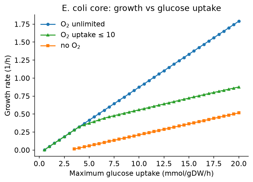

With glucose uptake capped at 10 mmol/gDW/h, the predicted growth rate is 0.874 h⁻¹ with oxygen and 0.212 h⁻¹ without it: aerobic respiration extracts far more ATP from each glucose than fermentation does. The growth curves show three more things.

• At zero glucose the problem is infeasible, not merely zero growth. With no carbon source, nothing can meet the ATP maintenance demand, so no flux vector satisfies all the constraints. The curves start only once glucose uptake covers maintenance, which takes more glucose without oxygen than with it.
• When glucose is the only limit, growth rises in a straight line. This is a general property of linear programs: scaling the one binding constraint scales the solution.
• When oxygen is also limited (the middle curve), the line bends at the point where oxygen runs out, and beyond it each extra unit of glucose buys less growth. A different constraint has become binding.

7.5 Exercises

1. In the toy network, raise the upper bound of \(v_6\) to 2000. Does the optimal growth change? Why not? What happens if you also raise the upper bound of \(b_2\)?
2. Remove the reaction R2 from the toy network (set both its bounds to 0) and rerun FVA. What happens to the ranges of \(v_1\) and \(v_3\), and why?
3. Run FVA on the E. coli core model under aerobic conditions (flux_variability_analysis in COBRApy, fluxVariability in the COBRA Toolbox). Which reactions can carry no flux at all? (Book, §8.8.1.)
4. At glucose uptake 10 and oxygen uptake at most 10 mmol/gDW/h, which by-products does the model secrete? Are they unique? Use FVA on the exchange reactions to find out.

7.6 Going further

The next chapter builds on these tools to study how networks respond to perturbations: gene and reaction knock-outs, synthetic lethals and over-expression (book, Chapters 9 and 10).

Orth, Jeffrey D., Ronan M. T. Fleming, and Bernhard Ø. Palsson. 2010. “Reconstruction and Use of Microbial Metabolic Networks: The Core Escherichia Coli Metabolic Model as an Educational Guide.” EcoSal Plus 4 (1). https://doi.org/10.1128/ecosalplus.10.2.1.