5 Boolean networks
ODE models need rate laws and parameters, and for gene regulatory and signalling networks these are rarely known. Often all we know is who activates or represses whom, and whether a gene is on or off. Boolean networks work at exactly that level: each gene is either ON (1) or OFF (0), time moves in discrete steps, and each gene’s next state is a logical function of the current states of its regulators. Such models have no parameters to estimate, and yet they can reproduce the qualitative behaviour of quite complex systems.
Chapter 7, Discrete Dynamic Models: Boolean Networks: transfer functions (§7.2), state transitions and attractors (§7.2.1), synchronous and asynchronous updates (§7.2.2), and other formalisms, from probabilistic Boolean networks to Petri nets (§7.3).
5.1 Transfer functions, states and attractors
A Boolean network of \(n\) variables is defined by a transfer function for each variable, built from AND, OR and NOT:
\[ X_i(t) = F_i\big(X_1(t-1), X_2(t-1), \ldots, X_n(t-1)\big). \]
With synchronous updating, as written here, all variables are updated at once from the previous state. The network then has \(2^n\) possible states, and each state has exactly one successor. Starting anywhere, the network must eventually revisit a state, and from then on it repeats itself. The states it repeats form an attractor: a single state that maps to itself (a steady state, or point attractor), or a cycle of states. The states that lead to an attractor form its basin.
For small networks, we can simply examine every state. Our first example is the three-gene network of the book’s Fig. 7.1:
\[ g_1^* = g_2 \text{ AND NOT } g_3, \qquad g_2^* = \text{NOT } g_1, \qquad g_3^* = (\text{NOT } g_3) \text{ OR } g_2, \]
where \(g_i^*\) is the next state of \(g_i\). States are written as three digits, \(g_1 g_2 g_3\); state 011, for example, has \(g_1\) OFF and \(g_2\), \(g_3\) ON.
Core MATLAB only.
%% A three-gene Boolean network (book Fig. 7.1, Eqs. 7.3)
%     g1* = g2 AND NOT g3
%     g2* = NOT g1
%     g3* = NOT g3 OR g2
% With synchronous updating, all genes are updated at once from the
% previous state. We list the successor of each of the 2^3 = 8 states,
% and find the attractors (the states the network ends up cycling
% through) and their basins (the states that lead to them).
% Requires: core MATLAB only.

n = 3;
update = @(x) [x(2) && ~x(3), ~x(1), ~x(3) || x(2)];
% State number <-> vector of 0/1, first gene as the leftmost digit
to_bits = @(s) bitget(s, n:-1:1);
to_number = @(x) sum(x .* 2.^(n-1:-1:0));
label = @(s) sprintf('%d', to_bits(s));

% Successor of every state (states are numbered 0 to 2^n - 1)
succ = zeros(1, 2^n);
for s = 0:2^n - 1
    succ(s + 1) = to_number(double(update(to_bits(s))));
    fprintf('%s => %s\n', label(s), label(succ(s + 1)));
end

% Attractors: follow each state until a state repeats; the repeating part
% is the attractor. Every state is assigned to the attractor it reaches.
attractors = {};
reaches = zeros(1, 2^n);
for s0 = 0:2^n - 1
    path = [];
    s = s0;
    while ~ismember(s, path)
        path(end + 1) = s; %#ok<AGROW>
        s = succ(s + 1);
    end
    cycle = path(find(path == s):end);
    key = min(cycle);
    if ~any(cellfun(@(a) min(a) == key, attractors))
        i = find(cycle == key);                     % start each cycle at
        attractors{end + 1} = cycle([i:end, 1:i - 1]); %#ok<SAGROW>
    end
    reaches(s0 + 1) = key;
end
basin_sizes = cellfun(@(a) sum(reaches == min(a)), attractors);
for k = 1:numel(attractors)
    a = attractors{k};
    fprintf('Attractor of period %d: %s; basin of %d states\n', numel(a), ...
        strjoin(arrayfun(label, a, 'UniformOutput', false), ' -> '), ...
        basin_sizes(k));
end

%% Plot the state transition map
labels = arrayfun(label, 0:2^n - 1, 'UniformOutput', false);
G = digraph(1:2^n, succ + 1, [], labels);   % MATLAB counts nodes from 1
% Same positions as the Python version, for states 000, 001, ..., 111
x = [3 1 2 3 0 1 0 2];
y = [1 1 1.5 0 1 0 0 0.5];
in_attractor = ismember(0:2^n - 1, [attractors{:}]);
fig = figure('Position', [100 100 700 350]);
h = plot(G, 'XData', x, 'YData', y, 'NodeLabel', labels, ...
    'MarkerSize', 12, 'NodeColor', 'k', 'EdgeColor', 'k', 'ArrowSize', 10);
highlight(h, find(in_attractor), 'NodeColor', [1.000 0.498 0.055]);
title('State transitions (orange: states in an attractor)');
axis off
sbp.save_figure(fig, mfilename('fullpath'), 'fig-three-genes');

results.successor = arrayfun(label, succ, 'UniformOutput', false);
results.attractors = cellfun(@(a) arrayfun(label, a, ...
    'UniformOutput', false), attractors, 'UniformOutput', false);
results.basin_sizes = basin_sizes;
sbp.save_results(mfilename('fullpath'), results);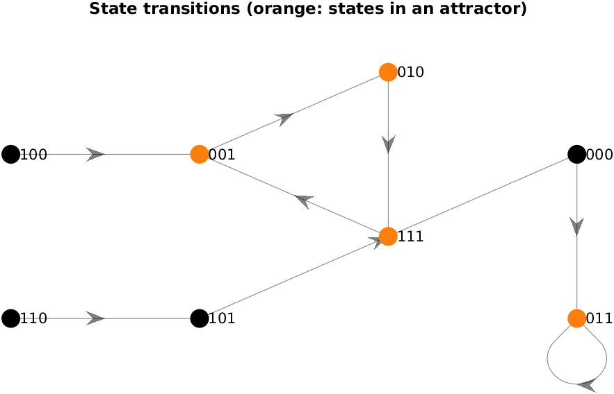
Needs NetworkX (for drawing the state transitions).
"""A three-gene Boolean network (book Fig. 7.1, Eqs. 7.3).

    g1* = g2 AND NOT g3
    g2* = NOT g1
    g3* = NOT g3 OR g2

With synchronous updating, all genes are updated at once from the
previous state. We list the successor of each of the 2^3 = 8 states,
and find the attractors (the states the network ends up cycling
through) and their basins (the states that lead to them).
"""
import numpy as np
import networkx as nx
import matplotlib.pyplot as plt
import sbp

genes = ["g1", "g2", "g3"]
n = len(genes)


def update(x):
    g1, g2, g3 = x
    return (g2 and not g3, not g1, (not g3) or g2)


def to_bits(s):
    """State number -> tuple of 0/1, first gene as the leftmost digit."""
    return tuple((s >> (n - 1 - i)) & 1 for i in range(n))


def to_number(x):
    return sum(int(b) << (n - 1 - i) for i, b in enumerate(x))


def label(s):
    return "".join(map(str, to_bits(s)))


# Successor of every state
succ = [to_number(update(to_bits(s))) for s in range(2 ** n)]
for s in range(2 ** n):
    print(f"{label(s)} => {label(succ[s])}")

# Attractors: follow each state until a state repeats; the repeating part
# is the attractor. Every state is assigned to the attractor it reaches.
attractor_of = {}
attractors = []
for s in range(2 ** n):
    path = []
    while s not in path:
        path.append(s)
        s = succ[s]
    cycle = path[path.index(s):]
    key = min(cycle)
    if key not in [min(a) for a in attractors]:
        i = cycle.index(key)                    # start each cycle at its
        attractors.append(cycle[i:] + cycle[:i])  # smallest state
    attractor_of[path[0]] = key
basins = {min(a): sum(1 for v in attractor_of.values() if v == min(a))
          for a in attractors}
for a in attractors:
    print(f"Attractor of period {len(a)}: "
          f"{' -> '.join(label(s) for s in a)}; basin of {basins[min(a)]} "
          f"states")

# --- Plot the state transition map
G = nx.DiGraph([(label(s), label(succ[s])) for s in range(2 ** n)])
pos = {"100": (0, 1), "110": (0, 0), "001": (1, 1), "101": (1, 0),
       "010": (2, 1.5), "111": (2, 0.5), "000": (3, 1), "011": (3, 0)}
in_attractor = {label(s) for a in attractors for s in a}
sbp.style()
fig, ax = plt.subplots(figsize=(7, 3.5))
nx.draw_networkx_nodes(G, pos, ax=ax, node_size=1100, edgecolors="k",
                       node_color=["#ff7f0e" if v in in_attractor else "white"
                                   for v in G.nodes])
nx.draw_networkx_labels(G, pos, ax=ax, font_size=11)
nx.draw_networkx_edges(G, pos, ax=ax, node_size=1100, arrowsize=18,
                       connectionstyle="arc3,rad=0.15")
ax.annotate("steady state\n(011 => 011)", pos["011"], xytext=(0, -38),
            textcoords="offset points", ha="center", va="top", fontsize=9)
ax.set_title("State transitions (orange: states in an attractor)")
ax.set_axis_off()
ax.margins(0.12)
sbp.save_figure(fig, __file__, "fig-three-genes")

sbp.save_results(__file__, {
    "successor": [label(s) for s in succ],
    "attractors": [[label(s) for s in a] for a in attractors],
    "basin_sizes": [basins[min(a)] for a in attractors],
})
sbp.show()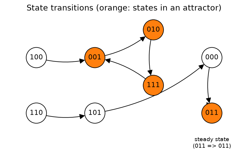
The transitions are those listed in the book (§7.2.1). The network has two attractors, each with a basin of four states: a steady state, 011, in which \(g_1\) stays off while \(g_2\) and \(g_3\) stay on; and a cycle of period three, 001 → 010 → 111 → 001, in which the genes switch on and off in a repeating pattern. Which of the two the network ends up in depends only on where it starts, and no state can reach both.
Following each state forward until it repeats, as the code does, finds every attractor of a synchronous network. With \(n\) variables there are \(2^n\) states to examine, which is quick up to \(n \approx 20\); beyond that, attractors must be sought by sampling starting states, or by specialised algorithms.
5.2 The mammalian cell cycle
The second example is a model of the mammalian cell cycle by Fauré and colleagues (Fauré et al. 2006), with ten variables: the cyclins CycD, CycE, CycA and CycB, the retinoblastoma protein Rb, the transcription factor E2F, the inhibitor p27, and the regulators Cdc20, Cdh1 and UbcH10 (Ubc). Its transfer functions are the book’s Eqs. 7.4. CycD stands for the growth signal: it has no regulators in the model, so it simply keeps its initial value.
With ten variables there are 1024 states, still few enough to examine every one. We do so twice. The first time with synchronous updating. The second time with asynchronous updating, which drops the assumption that every process takes exactly one time step: at each step, any one of the variables whose transfer function calls for a change may change, in any order. A state can then have several possible successors, so the states and their possible transitions form a directed graph, the state transition graph. An attractor is now a set of states that, once entered, can never be left: a strongly connected component of that graph with no transitions leading out of it, which graph libraries find directly.
Core MATLAB only.
%% A Boolean model of the mammalian cell cycle (Fauré et al., 2006)
% Ten genes and proteins; the update rules are the book's Eqs. 7.4. With
% 2^10 = 1024 possible states, we can examine every one of them:
%   1. synchronous updating, as in the previous example;
%   2. asynchronous updating, where one variable changes at a time, in
%      any order. The states then form a 'state transition graph', and the
%      attractors are the groups of states that, once entered, are never
%      left: its terminal strongly connected components.
% Requires: core MATLAB only.

names = {'CycD', 'Rb', 'E2F', 'CycE', 'CycA', 'p27', 'Cdc20', 'Cdh1', ...
         'Ubc', 'CycB'};
n = numel(names);
to_bits = @(s) double(bitget(s, n:-1:1));
to_number = @(x) sum(x .* 2.^(n-1:-1:0));

N = 2^n;
target = zeros(1, N);
for s = 0:N - 1
    target(s + 1) = to_number(double(update(to_bits(s))));
end

%% 1. Synchronous updating: follow every state to its attractor
keys = []; periods = []; reaches = zeros(1, N);
for s0 = 0:N - 1
    path = [];
    s = s0;
    while ~ismember(s, path)
        path(end + 1) = s; %#ok<AGROW>
        s = target(s + 1);
    end
    cycle = path(find(path == s):end);
    if ~ismember(min(cycle), keys)
        keys(end + 1) = min(cycle); %#ok<AGROW>
        periods(end + 1) = numel(cycle); %#ok<AGROW>
    end
    reaches(s0 + 1) = min(cycle);
end
[keys, order] = sort(keys);
periods = periods(order);
fprintf('Synchronous updating:\n');
for k = 1:numel(keys)
    b = to_bits(keys(k));
    sync_summary(k) = struct('period', periods(k), ...
        'basin', sum(reaches == keys(k)), 'CycD', b(1)); %#ok<SAGROW>
    fprintf('  attractor of period %d (CycD = %d), basin of %d states\n', ...
        periods(k), b(1), sync_summary(k).basin);
end

%% 2. Asynchronous updating: from each state, any one variable whose
% rule says it should change may change next
src = []; dst = [];
for s = 0:N - 1
    x = to_bits(s);
    fx = to_bits(target(s + 1));
    for i = find(x ~= fx)
        y = x;
        y(i) = fx(i);
        src(end + 1) = s + 1; %#ok<AGROW>
        dst(end + 1) = to_number(y) + 1; %#ok<AGROW>
    end
end
G = digraph(src, dst, [], N);
comp = conncomp(G, 'Type', 'strong');  % component of each state
C = condensation(G);                   % one node per component
terminal = find(outdegree(C) == 0)';
sizes = zeros(size(terminal)); cycd = zeros(size(terminal));
for k = 1:numel(terminal)
    members = find(comp == terminal(k)) - 1;  % back to states 0..N-1
    sizes(k) = numel(members);
    b = to_bits(min(members));
    cycd(k) = b(1);
end
[~, order] = sortrows([cycd' sizes']);
fprintf('Asynchronous updating:\n');
for k = 1:numel(order)
    async_summary(k) = struct('size', sizes(order(k)), ...
        'CycD', cycd(order(k))); %#ok<SAGROW>
    fprintf('  attractor of %d states (CycD = %d)\n', sizes(order(k)), ...
        cycd(order(k)));
end

%% A synchronous trajectory: start from a G1-like state, with CycD on
x0 = double(ismember(names, {'CycD', 'Rb', 'p27', 'Cdh1'}));
traj = zeros(21, n);
traj(1, :) = x0;
for t = 2:21
    traj(t, :) = double(update(traj(t - 1, :)));
end

fig = figure('Position', [100 100 800 360]);
imagesc(0:20, 1:n, traj', [0 1]);
colormap([0.97 0.98 1; 0.12 0.47 0.71]);   % OFF: light, ON: dark
set(gca, 'YTick', 1:n, 'YTickLabel', names, 'XTick', 0:2:20, 'Box', 'off');
xlabel('Time step');
title('Synchronous trajectory from a G1-like state (dark: ON, light: OFF)');
sbp.save_figure(fig, mfilename('fullpath'), 'fig-cell-cycle');

results.synchronous = sync_summary;
results.asynchronous = async_summary;
results.trajectory = traj;
sbp.save_results(mfilename('fullpath'), results);

%% Local function
function y = update(x)
% Book Eqs. 7.4 (Fauré et al., 2006)
x = num2cell(logical(x));
[CycD, Rb, E2F, CycE, CycA, p27, Cdc20, Cdh1, Ubc, CycB] = x{:};
y = [CycD, ...
     (~CycA && ~CycB && ~CycD && ~CycE) || (p27 && ~CycB && ~CycD), ...
     (~Rb && ~CycA && ~CycB) || (p27 && ~Rb && ~CycB), ...
     E2F && ~Rb, ...
     (E2F && ~Rb && ~Cdc20 && ~(Cdh1 && Ubc)) || ...
         (CycA && ~Rb && ~Cdc20 && ~(Cdh1 && Ubc)), ...
     (~CycD && ~CycE && ~CycA && ~CycB) || ...
         (p27 && ~(CycE && CycA) && ~CycB && ~CycD), ...
     CycB, ...
     (~CycA && ~CycB) || Cdc20 || (p27 && ~CycB), ...
     ~Cdh1 || (Cdh1 && Ubc && (Cdc20 || CycA || CycB)), ...
     ~Cdc20 && ~Cdh1];
end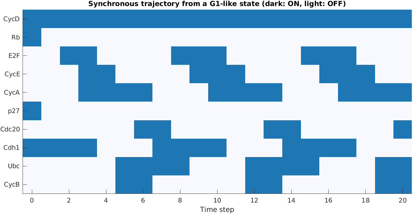
Needs NetworkX.
"""A Boolean model of the mammalian cell cycle (Fauré et al., 2006).

Ten genes and proteins; the update rules are the book's Eqs. 7.4. With
2^10 = 1024 possible states, we can examine every one of them:
  1. synchronous updating, as in the previous example;
  2. asynchronous updating, where one variable changes at a time, in
     any order. The states then form a 'state transition graph', and the
     attractors are the groups of states that, once entered, are never
     left: its terminal strongly connected components.
"""
import numpy as np
import networkx as nx
import matplotlib.pyplot as plt
import sbp

names = ["CycD", "Rb", "E2F", "CycE", "CycA", "p27", "Cdc20", "Cdh1",
         "Ubc", "CycB"]
n = len(names)


def update(x):
    CycD, Rb, E2F, CycE, CycA, p27, Cdc20, Cdh1, Ubc, CycB = x
    return (
        CycD,
        (not CycA and not CycB and not CycD and not CycE)
        or (p27 and not CycB and not CycD),
        (not Rb and not CycA and not CycB) or (p27 and not Rb and not CycB),
        E2F and not Rb,
        (E2F and not Rb and not Cdc20 and not (Cdh1 and Ubc))
        or (CycA and not Rb and not Cdc20 and not (Cdh1 and Ubc)),
        (not CycD and not CycE and not CycA and not CycB)
        or (p27 and not (CycE and CycA) and not CycB and not CycD),
        CycB,
        (not CycA and not CycB) or Cdc20 or (p27 and not CycB),
        (not Cdh1) or (Cdh1 and Ubc and (Cdc20 or CycA or CycB)),
        not Cdc20 and not Cdh1,
    )


def to_bits(s):
    return tuple((s >> (n - 1 - i)) & 1 for i in range(n))


def to_number(x):
    return sum(int(b) << (n - 1 - i) for i, b in enumerate(x))


states = range(2 ** n)
target = [to_number(update(to_bits(s))) for s in states]

# --- 1. Synchronous updating: follow every state to its attractor
sync_attractors = {}           # smallest state of the cycle -> cycle
reaches = []
for s in states:
    path = []
    while s not in path:
        path.append(s)
        s = target[s]
    cycle = path[path.index(s):]
    sync_attractors.setdefault(min(cycle), cycle)
    reaches.append(min(cycle))
sync_summary = [{"period": len(c), "basin": reaches.count(k),
                 "CycD": to_bits(k)[0]}
                for k, c in sorted(sync_attractors.items())]
print("Synchronous updating:")
for a in sync_summary:
    print(f"  attractor of period {a['period']} (CycD = {a['CycD']}), "
          f"basin of {a['basin']} states")

# --- 2. Asynchronous updating: from each state, any one variable whose
# rule says it should change may change next
G = nx.DiGraph()
G.add_nodes_from(states)
for s in states:
    x, fx = to_bits(s), to_bits(target[s])
    for i in range(n):
        if x[i] != fx[i]:
            y = list(x)
            y[i] = fx[i]
            G.add_edge(s, to_number(y))
C = nx.condensation(G)       # one node per strongly connected component
terminal = [c for c in C.nodes if C.out_degree(c) == 0]
async_summary = sorted(
    ({"size": len(C.nodes[c]["members"]),
      "CycD": to_bits(min(C.nodes[c]["members"]))[0]} for c in terminal),
    key=lambda a: (a["CycD"], a["size"]))
print("Asynchronous updating:")
for a in async_summary:
    print(f"  attractor of {a['size']} states (CycD = {a['CycD']})")

# --- A synchronous trajectory: start from a G1-like state, with CycD on
x0 = dict.fromkeys(names, 0)
x0.update(CycD=1, Rb=1, p27=1, Cdh1=1)
traj = [tuple(x0[g] for g in names)]
for _ in range(20):
    traj.append(tuple(int(v) for v in update(traj[-1])))
traj = np.array(traj)

sbp.style()
fig, ax = plt.subplots(figsize=(8, 3.6))
ax.imshow(traj.T, cmap="Blues", aspect="auto", vmin=0, vmax=1.3)
ax.set_yticks(range(n), names)
ax.set_xticks(range(0, 21, 2))
ax.set_xlabel("Time step")
ax.set_title("Synchronous trajectory from a G1-like state "
             "(dark: ON, light: OFF)")
for spine in ax.spines.values():
    spine.set_visible(False)
sbp.save_figure(fig, __file__, "fig-cell-cycle")

sbp.save_results(__file__, {
    "synchronous": sync_summary,
    "asynchronous": async_summary,
    "trajectory": traj,
})
sbp.show()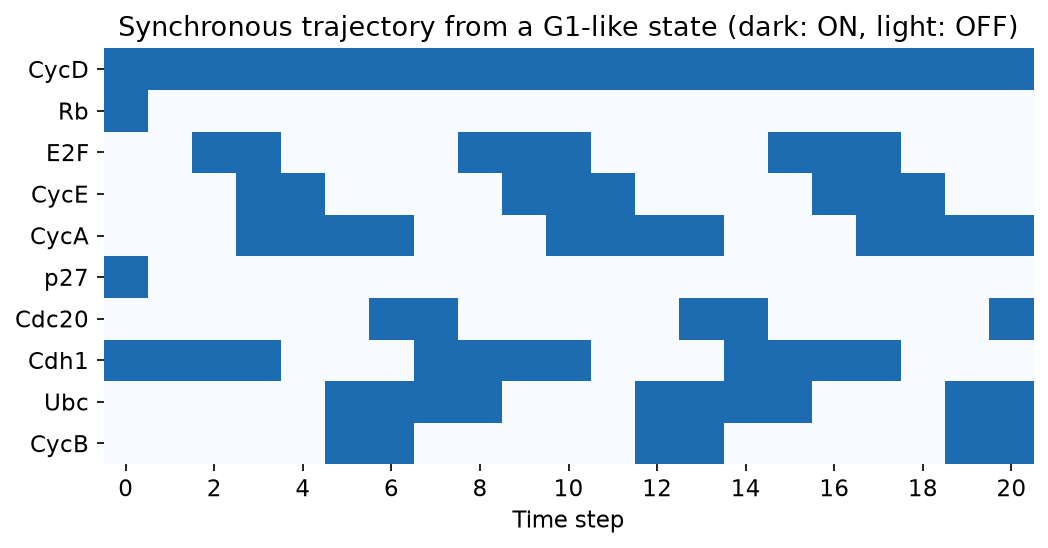
With synchronous updating, each half of the state space (CycD off, or CycD on) leads to a single attractor. Without the growth signal, the network settles into a steady state, a quiescent cell with Rb, p27 and Cdh1 active. With the growth signal, it settles into a cycle of seven states, in which E2F, then cyclin E, cyclin A and cyclin B rise and fall in turn, much as they do through the phases of a real cell cycle (figure). These are exactly the attractors reported by Fauré and colleagues.
Asynchronous updating keeps the quiescent steady state, but the seven-state cycle becomes a complex attractor of 112 states: the same sequence of events can now happen with many different relative timings, and the network wanders among all of them without ever leaving. Synchronous updating is easy to simulate and to reason about, but its fixed timing can create or destroy cycles that would not survive in a real cell; comparing both, as here, is a useful check on any conclusion drawn from a Boolean model (book, §7.5).
5.3 Exercises
- In the three-gene network, change the rule for \(g_3\) to \(g_3^* = (\text{NOT } g_3) \text{ AND } g_2\). Find the new attractors and their basins.
- Simulate a knock-out in the cell-cycle model: fix one variable at 0 (for example, Cdh1) and find the attractors again, with both kinds of updating. Which knock-outs abolish the cycle?
- Start the cell-cycle model in its quiescent steady state, switch CycD on, and update synchronously. Through which states does the network pass before it joins the seven-state cycle, and how many steps does that take?
- Write a function that generates a random Boolean network (Kauffman’s “NK” network): \(n\) genes, each with \(K\) randomly chosen regulators and a random truth table. For \(n = 12\) and \(K = 1, 2, 3, 4\), find the number of attractors and their periods, averaged over many networks. How does the behaviour change with \(K\)?
5.4 Going further
Boolean networks lie at one end of a spectrum of models. Between them and ODE models sit multi-valued logical models and Petri nets (book, §7.3). The next chapter returns to continuous quantities, but treats the small numbers of molecules inside a single cell as random events.