2  Networks

Many biological systems are naturally described as networks: proteins that bind one another, genes that regulate one another, metabolites linked by reactions. Before building detailed dynamic models of such systems, a great deal can be learnt from the structure of the network alone. This chapter computes the standard network parameters for a small example, and then generates the three classic network models, random, small-world and scale-free, to see how they differ.

NoteIn the book

Chapter 2, Introduction to Graph Theory: graphs, their representation as adjacency matrices and edge lists, and paths. Chapter 3, Structure of Networks: network parameters such as degree, clustering, path length and centrality (§3.1), and the canonical network models of Erdős and Rényi, Watts and Strogatz, and Barabási and Albert (§3.2). Communities, motifs and perturbations (§3.3–3.5) are left as exercises here.

2.1 Network parameters

A network, or graph, is a set of nodes joined by edges. For an undirected network of \(n\) nodes, the adjacency matrix \(\mathbf{A}\) has \(a_{ij} = 1\) if nodes \(i\) and \(j\) are joined, and 0 otherwise. Most network parameters follow directly from it:

• the degree \(k_i = \sum_j a_{ij}\), the number of neighbours of node \(i\);
• the clustering coefficient \(C_i\), the fraction of pairs of neighbours of \(i\) that are themselves joined. Because \((\mathbf{A}^3)_{ii}\) counts the closed walks of length three from \(i\), which is twice the number of triangles through \(i\), \(C_i = (\mathbf{A}^3)_{ii} / k_i(k_i - 1)\);
• the shortest-path length \(d_{ij}\) between every pair of nodes, from which follow the diameter (the largest \(d_{ij}\)) and the characteristic path length (the mean \(d_{ij}\) over all pairs);
• two measures of how central a node is: closeness, \((n-1)/\sum_j d_{ij}\), the reciprocal of the mean distance to all other nodes, and betweenness, the number of shortest paths between other pairs of nodes that pass through the node (a path shared by several equally short alternatives counts fractionally).

In MATLAB, networks are graph objects (or digraph for directed networks), part of core MATLAB. In Python, the standard package is NetworkX. Both provide shortest paths and centrality measures; we compute the clustering coefficient and closeness from their definitions, so that both languages use exactly the same formulas as the book.

Table 2.1: Working with networks in MATLAB and NetworkX.

	MATLAB	Python (NetworkX)
Build a network	G = graph(s, t)	G = nx.Graph(); G.add_edges_from(edges)
Adjacency matrix	adjacency(G) (sparse)	nx.to_numpy_array(G)
Degrees	degree(G)	dict(G.degree())
Shortest-path lengths	distances(G)	nx.floyd_warshall_numpy(G)
Betweenness	centrality(G, 'betweenness')	nx.betweenness_centrality(G, normalized=False)

Our example is a small network of ten proteins, two tightly knit groups joined through protein E.

MATLAB

Core MATLAB only.

%% Basic network parameters for a small undirected network
% Ten proteins, A to J, in two tightly knit groups joined through E.
% We compute degrees, clustering coefficients, shortest-path lengths and
% two centrality measures, using the definitions in the book (Ch. 3).
% Requires: core MATLAB only (graph objects, R2015b or newer).

nodes = cellstr(('A':'J')');
edges = {'A' 'B'; 'A' 'C'; 'A' 'D'; 'B' 'C'; 'B' 'D'; 'C' 'D'; 'D' 'E';
         'E' 'F'; 'F' 'G'; 'F' 'H'; 'G' 'H'; 'G' 'I'; 'H' 'I'; 'I' 'J'};
G = graph(edges(:, 1), edges(:, 2));
G = reordernodes(G, nodes);   % keep nodes in the order A, B, ..., J
n = numnodes(G);

% Adjacency matrix and degrees (book Eq. 3.1)
A = full(adjacency(G));
deg = sum(A, 2);

% Clustering coefficient (Eq. 3.6): the fraction of pairs of neighbours
% that are themselves connected; (A^3)_ii counts each triangle twice
triangles = diag(A^3) / 2;
pairs = deg .* (deg - 1) / 2;
clustering = zeros(n, 1);
clustering(pairs > 0) = triangles(pairs > 0) ./ pairs(pairs > 0);

% Shortest-path lengths between all pairs of nodes
D = distances(G);
diameter = max(D(:));                                  % Eq. 3.11
char_path_length = mean(D(triu(true(n), 1)));          % Eq. 3.12
closeness = (n - 1) ./ sum(D, 2);                      % Eq. 3.14

% Betweenness centrality (Eq. 3.17), counting each pair of nodes once
betweenness = centrality(G, 'betweenness');

fprintf('%d nodes, %d edges, mean degree %.2f\n', n, numedges(G), ...
    mean(deg));
fprintf(['mean clustering coefficient %.4f, diameter %g, ' ...
    'characteristic path length %.4f\n'], mean(clustering), diameter, ...
    char_path_length);
fprintf('node  degree  clustering  closeness  betweenness\n');
for i = 1:n
    fprintf('  %s   %4g    %8.3f   %8.3f   %9.2f\n', nodes{i}, deg(i), ...
        clustering(i), closeness(i), betweenness(i));
end

%% Plot: node size by degree, colour by betweenness, fixed positions
x = [0 1 0 1 2 3 4 3 4 5];
y = [1 1 0 0 0.5 0.5 1 0 0 0];
fig = figure('Position', [100 100 700 320]);
hold on
for e = 1:size(edges, 1)
    i = find(strcmp(nodes, edges{e, 1}));
    j = find(strcmp(nodes, edges{e, 2}));
    plot([x(i) x(j)], [y(i) y(j)], '-', 'Color', [0.6 0.6 0.6]);
end
scatter(x, y, 150 * deg, betweenness, 'filled', 'MarkerEdgeColor', 'k');
text(x, y + 0.12 + 0.03 * deg', nodes, 'HorizontalAlignment', 'center');
colormap(flipud(parula));
cb = colorbar;
cb.Label.String = 'Betweenness centrality';
title('Node size: degree; colour: betweenness');
axis off
ylim([-0.4 1.6]);
sbp.save_figure(fig, mfilename('fullpath'), 'fig-graph-basics');

results.degree = deg';
results.clustering = clustering';
results.mean_clustering = mean(clustering);
results.diameter = diameter;
results.char_path_length = char_path_length;
results.closeness = closeness';
results.betweenness = betweenness';
sbp.save_results(mfilename('fullpath'), results);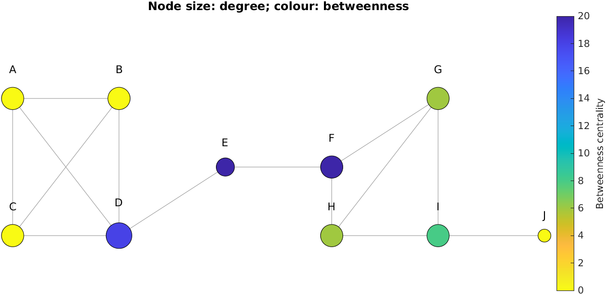

Python

Needs NetworkX.

"""Basic network parameters for a small undirected network.

Ten proteins, A to J, in two tightly knit groups joined through E.
We compute degrees, clustering coefficients, shortest-path lengths and
two centrality measures, using the definitions in the book (Ch. 3).
"""
import numpy as np
import networkx as nx
import matplotlib.pyplot as plt
import sbp

nodes = list("ABCDEFGHIJ")
edges = [("A", "B"), ("A", "C"), ("A", "D"), ("B", "C"), ("B", "D"),
         ("C", "D"), ("D", "E"), ("E", "F"), ("F", "G"), ("F", "H"),
         ("G", "H"), ("G", "I"), ("H", "I"), ("I", "J")]
G = nx.Graph()
G.add_nodes_from(nodes)
G.add_edges_from(edges)
n = G.number_of_nodes()

# Adjacency matrix and degrees (book Eq. 3.1)
A = nx.to_numpy_array(G, nodelist=nodes)
degree = A.sum(axis=1)

# Clustering coefficient (Eq. 3.6): the fraction of pairs of neighbours
# that are themselves connected; (A^3)_ii counts each triangle twice
triangles = np.diag(A @ A @ A) / 2
pairs = degree * (degree - 1) / 2
clustering = np.divide(triangles, pairs, out=np.zeros(n), where=pairs > 0)

# Shortest-path lengths between all pairs of nodes
D = nx.floyd_warshall_numpy(G, nodelist=nodes)
diameter = D.max()                                         # Eq. 3.11
char_path_length = D[np.triu_indices(n, k=1)].mean()      # Eq. 3.12
closeness = (n - 1) / D.sum(axis=1)                        # Eq. 3.14

# Betweenness centrality (Eq. 3.17), counting each pair of nodes once
bc = nx.betweenness_centrality(G, normalized=False)
betweenness = np.array([bc[v] for v in nodes])

print(f"{n} nodes, {G.number_of_edges()} edges, mean degree "
      f"{degree.mean():.2f}")
print(f"mean clustering coefficient {clustering.mean():.4f}, diameter "
      f"{diameter:g}, characteristic path length {char_path_length:.4f}")
print("node  degree  clustering  closeness  betweenness")
for i, v in enumerate(nodes):
    print(f"  {v}   {degree[i]:4g}    {clustering[i]:8.3f}   "
          f"{closeness[i]:8.3f}   {betweenness[i]:9.2f}")

# --- Plot: node size by degree, colour by betweenness, fixed positions
x = [0.0, 1.0, 0.0, 1.0, 2.0, 3.0, 4.0, 3.0, 4.0, 5.0]
y = [1.0, 1.0, 0.0, 0.0, 0.5, 0.5, 1.0, 0.0, 0.0, 0.0]
sbp.style()
fig, ax = plt.subplots(figsize=(7, 3.2))
idx = {v: i for i, v in enumerate(nodes)}
for u, w in edges:
    ax.plot([x[idx[u]], x[idx[w]]], [y[idx[u]], y[idx[w]]], "-",
            color="#999999", zorder=1)
sc = ax.scatter(x, y, s=150 * degree, c=betweenness, cmap="viridis_r",
                edgecolors="k", zorder=2)
for i, v in enumerate(nodes):
    ax.annotate(v, (x[i], y[i]), xytext=(0, 14 + 2 * degree[i]),
                textcoords="offset points", ha="center")
fig.colorbar(sc, ax=ax, label="Betweenness centrality")
ax.set_title("Node size: degree; colour: betweenness")
ax.set_axis_off()
ax.set_ylim(-0.4, 1.6)
sbp.save_figure(fig, __file__, "fig-graph-basics")

sbp.save_results(__file__, {
    "degree": degree, "clustering": clustering,
    "mean_clustering": clustering.mean(), "diameter": diameter,
    "char_path_length": char_path_length, "closeness": closeness,
    "betweenness": betweenness,
})
sbp.show()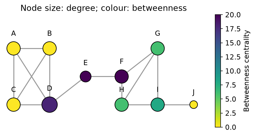

The different measures pick out different nodes. D has the largest degree, but E and F, with only two and three neighbours, carry the most shortest paths: every path between the two groups passes through both of them, so removing either would split the network in two. A, B and C, inside a complete group of four, have the highest clustering coefficient and no betweenness at all. Which measure matters depends on the question being asked; for example, betweenness, more than degree, often marks nodes whose removal disrupts communication across a network (book, §3.1.3 and §3.5).

2.2 Random and small-world networks

To judge whether a property of a real network is remarkable, we need something to compare it with. The simplest null model is the Erdős–Rényi random network, in which each of the \(\binom{n}{2}\) possible edges is present independently with probability \(p\). Its degrees follow a binomial distribution, close to a Poisson distribution for large \(n\); its clustering coefficient is about \(p\), which is very small for a sparse network; and its paths are short, growing only as \(\ln n\).

Real networks often combine short paths with high clustering. Watts and Strogatz showed how this can arise (Watts and Strogatz 1998). Start from a ring lattice, in which each node is joined to its \(k\) nearest neighbours on either side: clustering is high, but paths are long, since getting to the far side of the ring takes many steps. Then rewire each edge, with probability \(p\), to a randomly chosen node. The code below computes the mean clustering coefficient \(C(p)\) and characteristic path length \(L(p)\) as \(p\) rises from \(10^{-4}\) to 1, for networks of 500 nodes with ten neighbours each, averaging over ten networks at each \(p\). This is also the first problem of the BT5240 network assignment.

MATLAB

Core MATLAB only.

%% Small-world networks (Watts and Strogatz, 1998)
% Start from a ring lattice of n nodes, each linked to its k nearest
% neighbours on either side, and rewire each edge with probability p. A
% little rewiring makes paths short, as in a random network, while keeping
% the high clustering of the lattice. We also compare with Erdős–Rényi
% random networks with the same numbers of nodes and edges.
% Requires: core MATLAB only.

n = 500; k = 5;                   % 500 nodes, 2k = 10 neighbours each
probs = logspace(-4, 0, 13);      % rewiring probabilities
reps = 10;                        % networks averaged for each p
rng(1);

[C0, L0] = clustering_and_path_length(ring_lattice(n, k));
C = zeros(reps, numel(probs));
L = zeros(reps, numel(probs));
for r = 1:reps
    for i = 1:numel(probs)
        [C(r, i), L(r, i)] = clustering_and_path_length( ...
            watts_strogatz(n, k, probs(i)));
    end
end
C_ratio = mean(C, 1) / C0;
L_ratio = mean(L, 1) / L0;

p_er = n * k / (n * (n - 1) / 2);  % same expected number of edges, n*k
er = zeros(reps, 2);
for r = 1:reps
    [er(r, 1), er(r, 2)] = clustering_and_path_length(erdos_renyi(n, p_er));
end
er = mean(er, 1);

fprintf('Ring lattice: C = %.4f, L = %.4f\n', C0, L0);
for i = 1:numel(probs)
    fprintf('  p = %8.4f: C(p)/C(0) = %.3f, L(p)/L(0) = %.3f\n', ...
        probs(i), C_ratio(i), L_ratio(i));
end
fprintf('Erdős–Rényi, same n and m: C = %.4f, L = %.4f\n', er(1), er(2));

%% Plot
fig = figure;
semilogx(probs, C_ratio, 'o-', 'Color', [0.122 0.467 0.706]);
hold on
semilogx(probs, L_ratio, 's-', 'Color', [1.000 0.498 0.055]);
xlabel('Rewiring probability p'); ylabel('Relative to the ring lattice');
title(sprintf('Watts–Strogatz networks, n = %d, %d neighbours', n, 2 * k));
legend({'C(p) / C(0)', 'L(p) / L(0)'}, 'Location', 'southwest', ...
    'Box', 'off');
box off
sbp.save_figure(fig, mfilename('fullpath'), 'fig-small-world');

results.lattice = struct('C', C0, 'L', L0);
for p = [0.1 1]
    i = find(abs(probs - p) < 1e-12);
    name = strrep(sprintf('p_%g', p), '.', '_');
    results.ws.(name) = struct('C_ratio', C_ratio(i), ...
        'L_ratio', L_ratio(i));
end
results.er = struct('C', er(1), 'L', er(2));
results.probs = probs;
results.C_ratio = C_ratio;
results.L_ratio = L_ratio;
sbp.save_results(mfilename('fullpath'), results);

%% Local functions
function A = ring_lattice(n, k)
A = false(n);
idx = (1:n)';
for j = 1:k
    nb = mod(idx - 1 + j, n) + 1;
    A(sub2ind([n n], idx, nb)) = true;
    A(sub2ind([n n], nb, idx)) = true;
end
end

function A = watts_strogatz(n, k, p)
% Rewire each lattice edge (i, i+j) with probability p, moving its far
% end to a random node, avoiding self-loops and duplicate edges.
A = ring_lattice(n, k);
for j = 1:k
    for i = 1:n
        old = mod(i - 1 + j, n) + 1;
        if A(i, old) && rand < p
            new = randi(n);                 % draw until the new end is
            while new == i || A(i, new)     % neither i nor a neighbour
                new = randi(n);
            end
            A(i, old) = false; A(old, i) = false;
            A(i, new) = true;  A(new, i) = true;
        end
    end
end
end

function A = erdos_renyi(n, p)
upper = triu(rand(n) < p, 1);
A = upper | upper';
end

function [C, L] = clustering_and_path_length(A)
% Mean clustering coefficient, and mean shortest-path length over all
% pairs of nodes that are connected by some path.
A = double(A);
deg = sum(A, 2);
tri = sum((A * A) .* A, 2) / 2;
pairs = deg .* (deg - 1) / 2;
c = zeros(size(deg));
c(pairs > 0) = tri(pairs > 0) ./ pairs(pairs > 0);
C = mean(c);
D = distances(graph(A));
d = D(triu(true(size(A)), 1));
L = mean(d(isfinite(d)));
end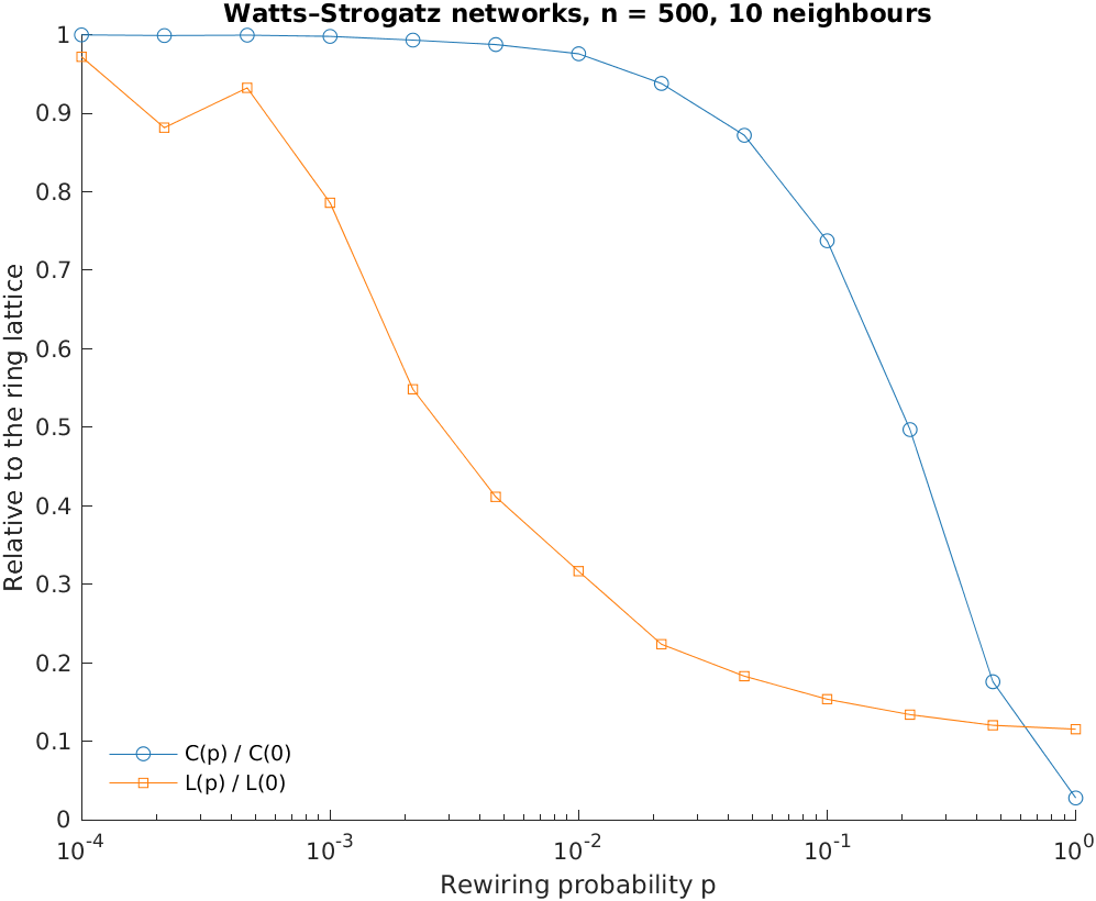

Python

Needs NumPy and SciPy.

"""Small-world networks (Watts and Strogatz, 1998).

Start from a ring lattice of n nodes, each linked to its k nearest
neighbours on either side, and rewire each edge with probability p. A
little rewiring makes paths short, as in a random network, while keeping
the high clustering of the lattice. We also compare with Erdős–Rényi
random networks with the same numbers of nodes and edges.
"""
import numpy as np
from scipy.sparse.csgraph import shortest_path
import matplotlib.pyplot as plt
import sbp

n, k = 500, 5                     # 500 nodes, 2k = 10 neighbours each
probs = np.logspace(-4, 0, 13)    # rewiring probabilities
reps = 10                         # networks averaged for each p
rng = np.random.default_rng(1)


def ring_lattice(n, k):
    A = np.zeros((n, n), dtype=bool)
    for j in range(1, k + 1):
        idx = np.arange(n)
        A[idx, (idx + j) % n] = A[(idx + j) % n, idx] = True
    return A


def watts_strogatz(n, k, p):
    """Rewire each lattice edge (i, i+j) with probability p, moving its far
    end to a random node, avoiding self-loops and duplicate edges."""
    A = ring_lattice(n, k)
    for j in range(1, k + 1):
        for i in range(n):
            old = (i + j) % n
            if A[i, old] and rng.random() < p:
                new = rng.integers(n)          # draw until the new end is
                while new == i or A[i, new]:   # neither i nor a neighbour
                    new = rng.integers(n)
                A[i, old] = A[old, i] = False
                A[i, new] = A[new, i] = True
    return A


def erdos_renyi(n, p):
    upper = np.triu(rng.random((n, n)) < p, 1)
    return upper | upper.T


def clustering_and_path_length(A):
    """Mean clustering coefficient, and mean shortest-path length over all
    pairs of nodes that are connected by some path."""
    A = A.astype(float)
    deg = A.sum(axis=1)
    tri = ((A @ A) * A).sum(axis=1) / 2
    pairs = deg * (deg - 1) / 2
    C = np.divide(tri, pairs, out=np.zeros(len(A)), where=pairs > 0).mean()
    D = shortest_path(A, unweighted=True, directed=False)
    d = D[np.triu_indices(len(A), k=1)]
    return C, d[np.isfinite(d)].mean()


C0, L0 = clustering_and_path_length(ring_lattice(n, k))
C, L = np.zeros((reps, probs.size)), np.zeros((reps, probs.size))
for r in range(reps):
    for i, p in enumerate(probs):
        C[r, i], L[r, i] = clustering_and_path_length(watts_strogatz(n, k, p))
C_ratio, L_ratio = C.mean(axis=0) / C0, L.mean(axis=0) / L0

p_er = n * k / (n * (n - 1) / 2)  # same expected number of edges, n*k
er = np.array([clustering_and_path_length(erdos_renyi(n, p_er))
               for _ in range(reps)]).mean(axis=0)

print(f"Ring lattice: C = {C0:.4f}, L = {L0:.4f}")
for p, c, l in zip(probs, C_ratio, L_ratio):
    print(f"  p = {p:8.4f}: C(p)/C(0) = {c:.3f}, L(p)/L(0) = {l:.3f}")
print(f"Erdős–Rényi, same n and m: C = {er[0]:.4f}, L = {er[1]:.4f}")

# --- Plot
sbp.style()
fig, ax = plt.subplots()
ax.semilogx(probs, C_ratio, "o-", color="#1f77b4", label="C(p) / C(0)")
ax.semilogx(probs, L_ratio, "s-", color="#ff7f0e", label="L(p) / L(0)")
ax.set_xlabel("Rewiring probability p")
ax.set_ylabel("Relative to the ring lattice")
ax.set_title(f"Watts–Strogatz networks, n = {n}, {2 * k} neighbours")
ax.legend(frameon=False, loc="lower left")
sbp.save_figure(fig, __file__, "fig-small-world")

at = {f"p_{p:g}".replace(".", "_"): i
      for i, p in enumerate(probs) if p in (0.1, 1.0)}
sbp.save_results(__file__, {
    "lattice": {"C": C0, "L": L0},
    "ws": {name: {"C_ratio": C_ratio[i], "L_ratio": L_ratio[i]}
           for name, i in at.items()},
    "er": {"C": er[0], "L": er[1]},
    "probs": probs, "C_ratio": C_ratio, "L_ratio": L_ratio,
})
sbp.show()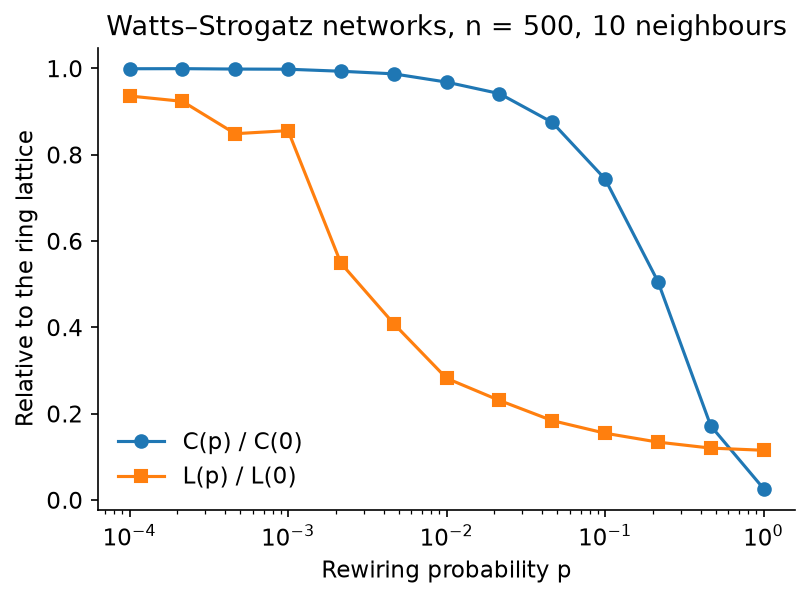

The two curves fall at very different rewiring probabilities. Rewiring 1% of the edges already shortens the typical path by about 70%, because each rewired edge is a shortcut across the ring, while clustering hardly changes, because each rewired edge removes only a few of the many triangles around it. Between \(p \approx 0.001\) and \(p \approx 0.1\), the networks are small worlds: clustered like a lattice, with paths almost as short as in a random network. At \(p = 1\), they are essentially random, and their clustering coefficient and path length are close to those of Erdős–Rényi networks with the same numbers of nodes and edges (about 0.02 and 2.9).

Since these networks are random, MATLAB and Python, which draw different random numbers, give slightly different results; the automated checks compare the averages, within 10%.

2.3 Scale-free networks

Erdős–Rényi and small-world networks share one feature that many biological networks do not: most nodes have roughly the same degree. In protein interaction and metabolic networks, by contrast, most nodes have very few neighbours while a few hubs have very many, and the degree distribution has a long tail, close to a power law, \(P(k) \propto k^{-\gamma}\). Such networks are called scale-free.

Barabási and Albert proposed a simple mechanism (Barabási and Albert 1999). The network grows one node at a time, and each new node attaches to \(m\) existing nodes, chosen with probability proportional to their degree: preferential attachment, or “the rich get richer”. For large networks this gives \(P(k) = 2m(m+1)/k(k+1)(k+2)\), which falls as \(k^{-3}\).

There is a neat way to choose a node with probability proportional to its degree: keep a list of the two ends of every edge, so that each node appears in it as many times as it has links, and pick an entry of that list uniformly at random.

MATLAB

Core MATLAB only.

%% Scale-free networks by preferential attachment (Barabási and Albert)
% Nodes are added one at a time; each new node links to m existing nodes,
% chosen with probability proportional to their degree. The resulting
% degree distribution has a heavy tail, P(k) ~ k^-3, with a few highly
% connected hubs. We compare it with an Erdős–Rényi network of the same
% size and mean degree.
% Requires: core MATLAB only.

n = 2000; m = 2;
reps = 10;
rng(1);

k_max = 200;
P_ba = zeros(1, k_max + 1); P_er = zeros(1, k_max + 1);
max_deg_ba = zeros(1, reps); max_deg_er = zeros(1, reps);
for r = 1:reps
    d = degrees(barabasi_albert(n, m), n);
    P_ba = P_ba + histcounts(min(d, k_max), -0.5:k_max + 0.5) / n / reps;
    max_deg_ba(r) = max(d);
    % Erdős–Rényi with the same expected mean degree
    mean_k = mean(d);
    upper = triu(rand(n) < mean_k / (n - 1), 1);
    d = sum(upper | upper', 2)';
    P_er = P_er + histcounts(min(d, k_max), -0.5:k_max + 0.5) / n / reps;
    max_deg_er(r) = max(d);
end

k = 0:k_max;
fprintf('Mean degree %.4f\n', mean_k);
fprintf(['Largest degree, averaged over %d networks: preferential ' ...
    'attachment %.1f, Erdős–Rényi %.1f\n'], reps, mean(max_deg_ba), ...
    mean(max_deg_er));
fprintf(['Fraction of nodes with degree >= 10: %.4f (theory for large ' ...
    'n: %.4f); Erdős–Rényi %.4f\n'], sum(P_ba(11:end)), ...
    m * (m + 1) / (10 * 11), sum(P_er(11:end)));

%% Plot. Right: the fraction of nodes with degree at least k, which is
% much less noisy in the tail than P(k) itself
ccdf_ba = fliplr(cumsum(fliplr(P_ba)));
ccdf_er = fliplr(cumsum(fliplr(P_er)));
blue = [0.122 0.467 0.706]; orange = [1.000 0.498 0.055];
fig = figure('Position', [100 100 1000 400]);
subplot(1, 2, 1)
plot(k, P_ba, 'o', 'Color', blue, 'MarkerFaceColor', blue, 'MarkerSize', 4);
hold on
plot(k, P_er, 's', 'Color', orange, 'MarkerFaceColor', orange, ...
    'MarkerSize', 4);
xlim([-0.5 30]);
xlabel('Degree k'); ylabel('Fraction of nodes with degree k');
title('Degree distribution');
legend({'preferential attachment', 'Erdős–Rényi'}, 'Box', 'off');
box off

subplot(1, 2, 2)
ok = ccdf_ba > 0 & k > 0;
loglog(k(ok), ccdf_ba(ok), 'o', 'Color', blue, 'MarkerFaceColor', blue, ...
    'MarkerSize', 4);
hold on
ok = ccdf_er > 0 & k > 0;
loglog(k(ok), ccdf_er(ok), 's', 'Color', orange, ...
    'MarkerFaceColor', orange, 'MarkerSize', 4);
kk = k(m + 1:end);
loglog(kk, m * (m + 1) ./ (kk .* (kk + 1)), '-', 'Color', [0.6 0.6 0.6]);
ylim([1e-5 1.5]);
xlabel('Degree k'); ylabel('Fraction of nodes with degree \geq k');
title('Tail, on logarithmic axes');
legend({'preferential attachment', 'Erdős–Rényi', ...
    'theory, m(m+1)/k(k+1)'}, 'Location', 'southwest', 'Box', 'off');
box off
sbp.save_figure(fig, mfilename('fullpath'), 'fig-scale-free');

results.mean_degree = mean_k;
results.ba = struct('P2', P_ba(3), 'P3', P_ba(4), ...
    'P_ge_10', sum(P_ba(11:end)), 'mean_max_degree', mean(max_deg_ba));
results.er = struct('mean_max_degree', mean(max_deg_er));
results.er_P_ge_10 = sum(P_er(11:end));
results.P_ba = P_ba(1:51);
results.P_er = P_er(1:51);
sbp.save_results(mfilename('fullpath'), results);

%% Local functions
function edges = barabasi_albert(n, m)
% Edge list of a preferential-attachment network. 'ends' lists every
% edge end, so a node appears in it once per link: picking a uniformly
% random element of 'ends' picks a node with probability proportional
% to its degree. Nodes are numbered from 0, as in the Python version.
n_edges = m * (m + 1) / 2 + m * (n - m - 1);
edges = zeros(n_edges, 2);
e = 0;
for i = 0:m                                % start from a clique
    for j = 0:i - 1
        e = e + 1;
        edges(e, :) = [i j];
    end
end
ends = reshape(edges(1:e, :)', 1, []);
ends = [ends, zeros(1, 2 * n_edges - numel(ends))];
n_ends = 2 * e;
for new = m + 1:n - 1
    targets = [];
    while numel(targets) < m
        t = ends(randi(n_ends));
        if ~ismember(t, targets)
            targets(end + 1) = t; %#ok<AGROW>
        end
    end
    for t = targets
        e = e + 1;
        edges(e, :) = [new t];
        ends(n_ends + 1:n_ends + 2) = [new t];
        n_ends = n_ends + 2;
    end
end
end

function d = degrees(edges, n)
d = accumarray(edges(:) + 1, 1, [n 1])';
end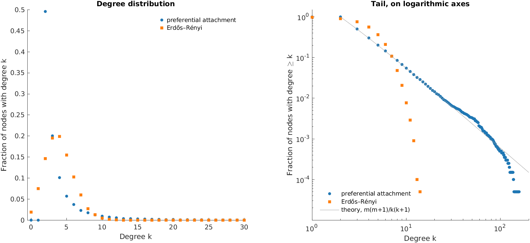

Python

Needs NumPy.

"""Scale-free networks by preferential attachment (Barabási and Albert).

Nodes are added one at a time; each new node links to m existing nodes,
chosen with probability proportional to their degree. The resulting
degree distribution has a heavy tail, P(k) ~ k^-3, with a few highly
connected hubs. We compare it with an Erdős–Rényi network of the same
size and mean degree.
"""
import numpy as np
import matplotlib.pyplot as plt
import sbp

n, m = 2000, 2
reps = 10
rng = np.random.default_rng(1)


def barabasi_albert(n, m):
    """Edge list of a preferential-attachment network. 'ends' lists every
    edge end, so a node appears in it once per link: picking a uniformly
    random element of 'ends' picks a node with probability proportional
    to its degree."""
    edges = [(i, j) for i in range(m + 1) for j in range(i)]  # a clique
    ends = [v for e in edges for v in e]
    for new in range(m + 1, n):
        targets = set()
        while len(targets) < m:
            targets.add(ends[rng.integers(len(ends))])
        for t in targets:
            edges.append((new, t))
            ends += [new, t]
    return edges


def degrees(edges, n):
    return np.bincount(np.ravel(edges), minlength=n)


k_max = 200
P_ba, P_er = np.zeros(k_max + 1), np.zeros(k_max + 1)
max_deg_ba, max_deg_er = [], []
for _ in range(reps):
    d = degrees(barabasi_albert(n, m), n)
    P_ba += np.bincount(np.minimum(d, k_max), minlength=k_max + 1) / n / reps
    max_deg_ba.append(d.max())
    # Erdős–Rényi with the same expected mean degree
    mean_k = d.mean()
    upper = np.triu(rng.random((n, n)) < mean_k / (n - 1), 1)
    d = (upper | upper.T).sum(axis=1)
    P_er += np.bincount(np.minimum(d, k_max), minlength=k_max + 1) / n / reps
    max_deg_er.append(d.max())

k = np.arange(k_max + 1)
print(f"Mean degree {mean_k:.4f}")
print(f"Largest degree, averaged over {reps} networks: preferential "
      f"attachment {np.mean(max_deg_ba):.1f}, Erdős–Rényi "
      f"{np.mean(max_deg_er):.1f}")
print(f"Fraction of nodes with degree >= 10: {P_ba[10:].sum():.4f} "
      f"(theory for large n: {m * (m + 1) / (10 * 11):.4f}); "
      f"Erdős–Rényi {P_er[10:].sum():.4f}")

# --- Plot. Right: the fraction of nodes with degree at least k, which is
# much less noisy in the tail than P(k) itself
ccdf_ba, ccdf_er = P_ba[::-1].cumsum()[::-1], P_er[::-1].cumsum()[::-1]
sbp.style()
fig, (ax1, ax2) = plt.subplots(1, 2, figsize=(10, 4))
ax1.plot(k, P_ba, "o", color="#1f77b4", ms=4, label="preferential attachment")
ax1.plot(k, P_er, "s", color="#ff7f0e", ms=4, label="Erdős–Rényi")
ax1.set_xlim(-0.5, 30)
ax1.set_xlabel("Degree k")
ax1.set_ylabel("Fraction of nodes with degree k")
ax1.set_title("Degree distribution")
ax1.legend(frameon=False)
ax2.loglog(k[1:][ccdf_ba[1:] > 0], ccdf_ba[1:][ccdf_ba[1:] > 0], "o",
           color="#1f77b4", ms=4, label="preferential attachment")
ax2.loglog(k[1:][ccdf_er[1:] > 0], ccdf_er[1:][ccdf_er[1:] > 0], "s",
           color="#ff7f0e", ms=4, label="Erdős–Rényi")
ax2.loglog(k[m:], m * (m + 1) / (k[m:] * (k[m:] + 1.0)), "-",
           color="#999999", label="theory, $m(m+1)/k(k+1)$")
ax2.set_ylim(1e-5, 1.5)
ax2.set_xlabel("Degree k")
ax2.set_ylabel("Fraction of nodes with degree $\\geq$ k")
ax2.set_title("Tail, on logarithmic axes")
ax2.legend(frameon=False, loc="lower left")
sbp.save_figure(fig, __file__, "fig-scale-free")

sbp.save_results(__file__, {
    "mean_degree": mean_k,
    "ba": {"P2": P_ba[2], "P3": P_ba[3], "P_ge_10": P_ba[10:].sum(),
           "mean_max_degree": np.mean(max_deg_ba)},
    "er": {"mean_max_degree": np.mean(max_deg_er)},
    "er_P_ge_10": P_er[10:].sum(),
    "P_ba": P_ba[:51], "P_er": P_er[:51],
})
sbp.show()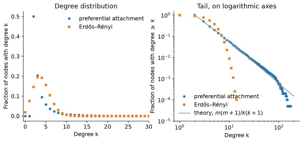

Both networks have 2000 nodes and a mean degree of about four. In the random network, no node has more than about a dozen neighbours. With preferential attachment, half of the nodes have only the minimum two links, and the most connected node has, on average over ten networks, more than a hundred. On logarithmic axes the tail of the distribution follows the predicted straight line until it runs out of nodes.

Plotting the fraction of nodes with degree at least \(k\) (right panel), in place of the fraction with degree exactly \(k\), avoids most of the noise in the tail, where only one or two nodes have each degree. Even so, deciding whether a real network is truly scale-free from a straight-looking line on a log–log plot is risky; the book discusses better tests (§3.6.1).

2.4 Exercises

1. Remove node E from the example network. Recompute all the parameters. What happens to the diameter, and why do the shortest-path functions report infinite distances?
2. Generate Erdős–Rényi networks with \(n = 1000\) and mean degree from 0.2 to 3. Plot the size of the largest connected component (conncomp in MATLAB, nx.connected_components in Python) against the mean degree. What happens at a mean degree of 1?
3. For the scale-free network, remove nodes one at a time, either at random or in order of decreasing degree, and track the size of the largest connected component. Repeat for the Erdős–Rényi network. Which network is more robust to random failures, and which to targeted attack (book, §3.5.2)?
4. Download a biological network, for example a protein interaction network from https://networkrepository.com/, and compute its degree distribution, mean clustering coefficient and characteristic path length. Compare them with an Erdős–Rényi network with the same numbers of nodes and edges. (This is the second problem of the BT5240 network assignment.)
5. The book’s code repository has a function barabasi_albert.m for \(m = 1\). What kind of network does it always produce, and what is its clustering coefficient?

2.5 Going further

Detecting communities and network motifs (book, §3.3–3.4) builds on the same tools, together with randomised networks that preserve each node’s degree. Chapter 4 of the book applies these ideas to biological questions, from predicting essential genes to finding disease modules.

Barabási, Albert-László, and Réka Albert. 1999. “Emergence of Scaling in Random Networks.” Science 286 (5439): 509–12. https://doi.org/10.1126/science.286.5439.509.

Watts, Duncan J., and Steven H. Strogatz. 1998. “Collective Dynamics of ‘Small-World’ Networks.” Nature 393: 440–42. https://doi.org/10.1038/30918.