4 Parameter estimation
Every dynamic model carries parameters, such as rate constants, Michaelis constants and inhibition constants, and only a few of them can be looked up. The rest must be estimated from experimental data: we look for the parameter values that make the model’s predictions agree best with the measurements. This chapter sets up that problem for a small enzyme-kinetic model, solves it in three different ways, and shows what the data can and cannot tell us about the parameters.
Chapter 6, Parameter Estimation: least squares and its weighted forms (§6.2.2), maximum likelihood (§6.2.3), algorithms for optimisation, from direct search to evolutionary algorithms (§6.3), post-regression diagnostics (§6.4) and troubleshooting, including identifiability and the curse of dimensionality (§6.5). Exercise 6.1 uses the same model.
4.1 The model and the data
An enzyme follows Michaelis–Menten kinetics with a competitive inhibitor \(I\):
\[ v = \frac{v_\text{max}\,S}{K_M\left(1 + \dfrac{I}{K_I}\right) + S}. \]
We want \(v_\text{max}\), \(K_M\) and \(K_I\). The initial rate \(v\) was measured at 20 substrate concentrations, from 1 to 20 mM, once with the inhibitor at \(I = 10\) mM (dataset D1) and once at \(I = 20\) mM (dataset D2). The data are in data/competitive_inhibition.csv.
Each measurement is assumed to carry an error of about 10% of its value, \(\delta = 0.1\). A good fit should therefore be judged by relative errors, and the cost we minimise is the weighted sum of squared errors (book, Eq. 6.5):
\[ \text{SSE}(\Theta) = \sum_{i=1}^{n} \left( \frac{v_{\text{pred},i}(\Theta) - v_i}{\delta\, v_i} \right)^2, \qquad \Theta = (v_\text{max}, K_M, K_I). \]
If the measurement errors are independent and normally distributed with standard deviation \(\delta v_i\), minimising this SSE is the same as finding the maximum-likelihood estimate (book, §6.2.3).
4.2 Fitting by least squares
Both MATLAB and SciPy have solvers made for least-squares problems. They take a function that returns the vector of weighted residuals, one per data point, and minimise the sum of their squares. They use the structure of the problem to converge quickly, but, like all local methods, they need a starting guess.
| MATLAB | Python (SciPy) | |
|---|---|---|
| Least squares (residual vector) | lsqnonlin (Optimization Toolbox) |
scipy.optimize.least_squares |
| General minimisation, no derivatives | fminsearch (core MATLAB) |
scipy.optimize.minimize(method="Nelder-Mead") |
| Global search | ga, particleswarm (Global Optimization Toolbox) |
scipy.optimize.differential_evolution |
We fit each dataset, D1, D2 and both together, from the same eight starting guesses.
Needs the Optimization Toolbox (for lsqnonlin).
%% Fitting a rate law to data by weighted least squares
% Competitive inhibition:  v = vmax*S / (KM*(1 + I/KI) + S).
% Rates were measured at 20 substrate concentrations, with the inhibitor
% at I = 10 mM (dataset D1) and at I = 20 mM (dataset D2). We estimate
% vmax, KM and KI from D1 alone, and from both datasets together.
% Requires: Optimization Toolbox (for lsqnonlin).

data = readmatrix(fullfile(sbp.data_dir(), 'competitive_inhibition.csv'));
S = data(:, 1); v10 = data(:, 2); v20 = data(:, 3);
delta = 0.1;                      % relative measurement error (10%)

rate = @(p, S, I) p(1) * S ./ (p(2) * (1 + I / p(3)) + S);
% Weighted residuals; their sum of squares is the SSE (book Eq. 6.5)
residuals = @(p, S, I, v) (rate(p, S, I) - v) ./ (delta * v);
opts = optimoptions('lsqnonlin', 'Display', 'off', ...
    'StepTolerance', 1e-12, 'FunctionTolerance', 1e-12, ...
    'OptimalityTolerance', 1e-12);

% The same eight starting guesses for every fit: vmax = 20 and a spread
% of values for KM and KI
KM_KI = [1 1; 2 8; 5 2; 5 20; 10 5; 20 40; 40 10; 40 80];
starts = [20 * ones(8, 1), KM_KI];

names = {'D1', 'D2', 'D1_D2'};
datasets = {{S, 10 * ones(20, 1), v10}, ...
            {S, 20 * ones(20, 1), v20}, ...
            {[S; S], [10 * ones(20, 1); 20 * ones(20, 1)], [v10; v20]}};

for d = 1:3
    [s, i, v] = datasets{d}{:};
    P = zeros(8, 3);
    SSE = zeros(8, 1);
    for k = 1:8
        [P(k, :), SSE(k)] = lsqnonlin(@(p) residuals(p, s, i, v), ...
            starts(k, :), [0 0 0], [Inf Inf Inf], opts);
    end
    [~, best] = min(SSE);
    % KM*(1 + I/KI) at the first inhibitor level of the dataset
    KM_app = P(:, 2) .* (1 + i(1) ./ P(:, 3));
    fprintf('%s: SSE = %.4f (spread over starts %.1e)\n', names{d}, ...
        SSE(best), max(SSE) - min(SSE));
    fprintf(['   vmax = %.4f;  KM ranges %.3g to %.3g;  ' ...
        'KI ranges %.3g to %.3g\n'], P(best, 1), min(P(:, 2)), ...
        max(P(:, 2)), min(P(:, 3)), max(P(:, 3)));
    % What every start agrees on; KM and KI only if they are pinned down
    results.(names{d}) = struct('SSE', SSE(best), 'vmax', P(best, 1), ...
        'KM_app', KM_app(best));
    if strcmp(names{d}, 'D1_D2')
        results.D1_D2.KM = P(best, 2);
        results.D1_D2.KI = P(best, 3);
    else
        results.([names{d} '_estimates']) = struct('KM', P(:, 2)', ...
            'KI', P(:, 3)');
    end
end

%% Plot
fig = figure('Position', [100 100 1000 400]);
blue = [0.122 0.467 0.706]; orange = [1.000 0.498 0.055];
r = results.D1_D2;
p = [r.vmax r.KM r.KI];
S_fine = linspace(0, 21, 200);

subplot(1, 2, 1)
hold on
errorbar(S, v10, delta * v10, 'o', 'Color', blue, 'MarkerSize', 4, ...
    'MarkerFaceColor', blue);
errorbar(S, v20, delta * v20, 'o', 'Color', orange, 'MarkerSize', 4, ...
    'MarkerFaceColor', orange);
plot(S_fine, rate(p, S_fine, 10), '-', 'Color', blue);
plot(S_fine, rate(p, S_fine, 20), '-', 'Color', orange);
xlabel('S (mM)'); ylabel('v (mmol L^{-1} s^{-1})');
title('Fit to D1 and D2 together');
legend({'data, I = 10 mM', 'data, I = 20 mM'}, 'Location', 'southeast', ...
    'Box', 'off');
box off

subplot(1, 2, 2)
KI_line = logspace(-1, 2.3, 200);
loglog(results.D1.KM_app ./ (1 + 10 ./ KI_line), KI_line, '-', ...
    'Color', [0.6 0.6 0.6]);
hold on
est = results.D1_estimates;
loglog(est.KM, est.KI, 'o', 'Color', blue, 'MarkerFaceColor', blue);
loglog(p(2), p(3), 'p', 'Color', [0.839 0.153 0.157], ...
    'MarkerFaceColor', [0.839 0.153 0.157], 'MarkerSize', 14);
xlabel('K_M (mM)'); ylabel('K_I (mM)');
title('Where the estimates land');
legend({'K_M(1 + 10/K_I) = best K_M^{app} for D1', ...
    'estimates from D1, 8 starts', 'estimate from D1 and D2'}, ...
    'Location', 'northwest', 'Box', 'off', 'FontSize', 9);
box off
sbp.save_figure(fig, mfilename('fullpath'), 'fig-fit-inhibition');

sbp.save_results(mfilename('fullpath'), results);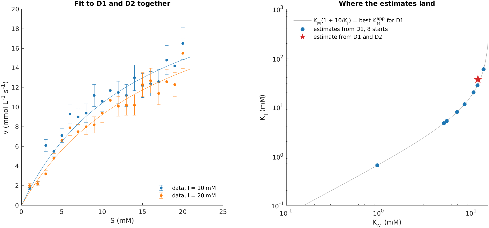
Needs SciPy.
"""Fitting a rate law to data by weighted least squares.

Competitive inhibition:  v = vmax*S / (KM*(1 + I/KI) + S).
Rates were measured at 20 substrate concentrations, with the inhibitor
at I = 10 mM (dataset D1) and at I = 20 mM (dataset D2). We estimate
vmax, KM and KI from D1 alone, and from both datasets together.
"""
import numpy as np
from scipy.optimize import least_squares
import matplotlib.pyplot as plt
import sbp

data = np.loadtxt(sbp.DATA / "competitive_inhibition.csv", delimiter=",",
                  skiprows=1)
S, v10, v20 = data[:, 0], data[:, 1], data[:, 2]
delta = 0.1                       # relative measurement error (10%)


def rate(p, S, I):
    vmax, KM, KI = p
    return vmax * S / (KM * (1 + I / KI) + S)


def residuals(p, S, I, v):
    """Weighted residuals; their sum of squares is the SSE (book Eq. 6.5)."""
    return (rate(p, S, I) - v) / (delta * v)


def fit(S, I, v, p0):
    sol = least_squares(residuals, p0, args=(S, I, v), bounds=(0, np.inf),
                        xtol=1e-12, ftol=1e-12, gtol=1e-12)
    return sol.x, np.sum(sol.fun ** 2)


# The same eight starting guesses for every fit: vmax = 20 and a spread
# of values for KM and KI
starts = [(20, km, ki) for km, ki in
          [(1, 1), (2, 8), (5, 2), (5, 20), (10, 5), (20, 40), (40, 10),
           (40, 80)]]

datasets = {
    "D1": (S, np.full_like(S, 10.0), v10),
    "D2": (S, np.full_like(S, 20.0), v20),
    "D1_D2": (np.r_[S, S], np.r_[np.full_like(S, 10.0),
                                  np.full_like(S, 20.0)], np.r_[v10, v20]),
}

results = {}
for name, (s, i, v) in datasets.items():
    fits = [fit(s, i, v, p0) for p0 in starts]
    P = np.array([p for p, _ in fits])
    SSE = np.array([sse for _, sse in fits])
    best = np.argmin(SSE)
    # KM*(1 + I/KI) at the first inhibitor level of the dataset
    KM_app = P[:, 1] * (1 + i[0] / P[:, 2])
    print(f"{name}: SSE = {SSE[best]:.4f} (spread over starts "
          f"{np.ptp(SSE):.1e})")
    print(f"   vmax = {P[best, 0]:.4f};  KM ranges {P[:, 1].min():.3g} to "
          f"{P[:, 1].max():.3g};  KI ranges {P[:, 2].min():.3g} to "
          f"{P[:, 2].max():.3g}")
    # What every start agrees on; KM and KI only if they are pinned down
    results[name] = {"SSE": SSE[best], "vmax": P[best, 0],
                     "KM_app": KM_app[best]}
    if name == "D1_D2":
        results[name].update(KM=P[best, 1], KI=P[best, 2])
    else:
        results[name + "_estimates"] = {"KM": P[:, 1], "KI": P[:, 2]}

# --- Plot
sbp.style()
fig, (ax1, ax2) = plt.subplots(1, 2, figsize=(10, 4))
p = [results["D1_D2"][k] for k in ("vmax", "KM", "KI")]
S_fine = np.linspace(0, 21, 200)
for I, v, col in [(10, v10, "#1f77b4"), (20, v20, "#ff7f0e")]:
    ax1.errorbar(S, v, yerr=delta * v, fmt="o", color=col, ms=4,
                 capsize=2, label=f"data, I = {I} mM")
    ax1.plot(S_fine, rate(p, S_fine, I), "-", color=col)
ax1.set_xlabel("S (mM)")
ax1.set_ylabel("v (mmol L$^{-1}$ s$^{-1}$)")
ax1.set_title("Fit to D1 and D2 together")
ax1.legend(frameon=False, loc="lower right")

KI_line = np.logspace(-1, 2.3, 200)
ax2.plot(results["D1"]["KM_app"] / (1 + 10 / KI_line), KI_line, "-",
         color="#999999", label="$K_M(1 + 10/K_I)$ = best $K_M^{app}$ for D1")
est = results["D1_estimates"]
ax2.plot(est["KM"], est["KI"], "o", color="#1f77b4", ms=6,
         label="estimates from D1, 8 starts")
ax2.plot(p[1], p[2], "*", color="#d62728", ms=14,
         label="estimate from D1 and D2")
ax2.set_xscale("log")
ax2.set_yscale("log")
ax2.set_xlabel("$K_M$ (mM)")
ax2.set_ylabel("$K_I$ (mM)")
ax2.set_title("Where the estimates land")
ax2.legend(frameon=False, loc="upper left", fontsize=9)
sbp.save_figure(fig, __file__, "fig-fit-inhibition")

sbp.save_results(__file__, results)
sbp.show()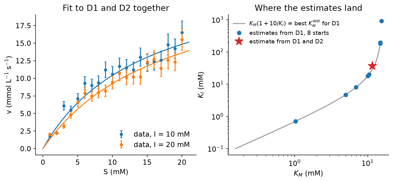
With both datasets, all eight starts arrive at the same answer, \(v_\text{max} = 25.8\) mmol L−1 s−1, \(K_M = 11.6\) mM and \(K_I = 36.8\) mM, and the curves follow the data well (left panel).
With D1 alone, something quite different happens. All eight starts again reach exactly the same SSE and the same \(v_\text{max}\), and every one of them reports a successful fit. Yet \(K_M\) ranges from about 1 to 15 mM and \(K_I\) from below 1 to several hundred mM. The right panel shows why. At a single inhibitor concentration, \(K_M\) and \(K_I\) enter the rate law only through the combination
\[ K_M^\text{app} = K_M\left(1 + \frac{I}{K_I}\right), \]
the apparent Michaelis constant. Every pair \((K_M, K_I)\) on the grey curve gives the same \(K_M^\text{app}\), and hence identical predictions for every data point. The data determine \(v_\text{max}\) and \(K_M^\text{app}\), and nothing more: \(K_M\) and \(K_I\) are structurally non-identifiable from D1. More data of the same kind would not help. A second inhibitor concentration does, because \(K_M^\text{app}\) changes with \(I\) in a way that depends on \(K_I\) (red star).
Two lessons follow. First, a solver that reports success has found a minimum; it says nothing about whether the minimum is unique. Fitting from several starting points is a simple and effective check. Second, identifiability is a property of the model and the experiment together, and it is best examined before the experiments are done (book, §6.5.3).
4.3 The error landscape, and grid search
The simplest way to minimise a function is to evaluate it everywhere, on a grid, and keep the best point (book, §6.3.3). Grid search needs no starting guess and cannot be trapped by a local minimum, and it shows the whole error landscape, which makes it a good tool for seeing what is going on.
Here, one more trick keeps the grid small. The rate law is proportional to \(v_\text{max}\), so for given \(K_M\) and \(K_I\) the weighted residuals are linear in \(v_\text{max}\), and the best \(v_\text{max}\) follows from a one-line formula, just as in linear regression. The search is then over \(K_M\) and \(K_I\) only: whole numbers from 1 to 60 mM, 3600 points.
Core MATLAB only.
%% Grid search, and the shape of the error landscape
% The same competitive-inhibition model and data as in fit_inhibition.
% We evaluate the weighted SSE on a grid of whole-number values of KM and
% KI (1 to 60 mM). The rate is proportional to vmax, so for each (KM, KI)
% the best vmax can be computed exactly, as in linear regression, and the
% grid only needs two dimensions.
% Requires: core MATLAB only.

data = readmatrix(fullfile(sbp.data_dir(), 'competitive_inhibition.csv'));
S = data(:, 1); v10 = data(:, 2); v20 = data(:, 3);
delta = 0.1;
names = {'D1', 'D1_D2'};
datasets = {{S, 10 * ones(20, 1), v10}, ...
            {[S; S], [10 * ones(20, 1); 20 * ones(20, 1)], [v10; v20]}};
KM_grid = 1:60;
KI_grid = 1:60;

for d = 1:2
    [s, i, v] = datasets{d}{:};
    grid = zeros(numel(KI_grid), numel(KM_grid));  % rows: KI, columns: KM
    vmax = zeros(size(grid));
    for r = 1:numel(KI_grid)
        for c = 1:numel(KM_grid)
            [vmax(r, c), grid(r, c)] = best_vmax_and_sse( ...
                KM_grid(c), KI_grid(r), s, i, v, delta);
        end
    end
    [best, idx] = min(grid(:));
    [r, c] = ind2sub(size(grid), idx);
    % How many grid points fit almost as well as the best (within 1 unit)?
    n_close = sum(grid(:) < best + 1);
    fprintf(['%s: best on grid KM = %d, KI = %d, vmax = %.4f, ' ...
        'SSE = %.4f; %d grid points within 1 of the best SSE\n'], ...
        names{d}, KM_grid(c), KI_grid(r), vmax(r, c), best, n_close);
    SSE.(names{d}) = grid;
    results.(names{d}) = struct('KM', KM_grid(c), 'KI', KI_grid(r), ...
        'vmax', vmax(r, c), 'SSE', best, 'n_within_1', n_close, ...
        'SSE_at_KI_20', grid(KI_grid == 20, :));
end

%% Plot: log10(SSE - best SSE + 1), so that the best point is at 0
fig = figure('Position', [100 100 1000 420]);
titles = {'D1 only (I = 10 mM)', 'D1 and D2 together'};
for d = 1:2
    subplot(1, 2, d)
    Z = log10(SSE.(names{d}) - min(SSE.(names{d})(:)) + 1);
    contourf(KM_grid, KI_grid, min(Z, 3), linspace(0, 3, 13), ...
        'LineStyle', 'none');
    hold on
    plot(results.(names{d}).KM, results.(names{d}).KI, 'p', ...
        'Color', [0.839 0.153 0.157], ...
        'MarkerFaceColor', [0.839 0.153 0.157], 'MarkerSize', 14);
    colormap(flipud(parula));
    clim([0 3]);
    xlabel('K_M (mM)');
    if d == 1, ylabel('K_I (mM)'); end
    title(titles{d});
end
cb = colorbar;
cb.Label.String = 'log_{10}(SSE - best SSE + 1)';
sbp.save_figure(fig, mfilename('fullpath'), 'fig-sse-landscape');

sbp.save_results(mfilename('fullpath'), results);

%% Local function
function [vmax, sse] = best_vmax_and_sse(KM, KI, S, I, v, delta)
% Weighted residuals are vmax*a - b, so the best vmax is sum(a.*b)/sum(a.^2).
a = S ./ (KM * (1 + I / KI) + S) ./ (delta * v);
b = 1 / delta;
vmax = sum(a .* b) / sum(a .* a);
sse = sum((vmax * a - b) .^ 2);
end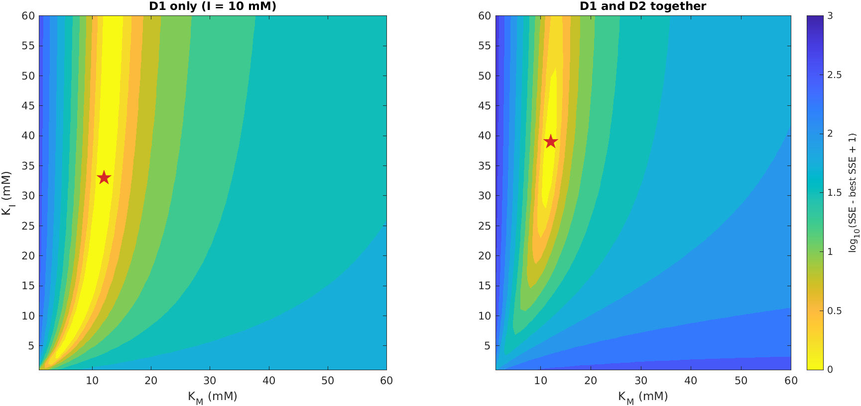
Needs NumPy and Matplotlib.
"""Grid search, and the shape of the error landscape.

The same competitive-inhibition model and data as in fit_inhibition.
We evaluate the weighted SSE on a grid of whole-number values of KM and
KI (1 to 60 mM). The rate is proportional to vmax, so for each (KM, KI)
the best vmax can be computed exactly, as in linear regression, and the
grid only needs two dimensions.
"""
import numpy as np
import matplotlib.pyplot as plt
import sbp

data = np.loadtxt(sbp.DATA / "competitive_inhibition.csv", delimiter=",",
                  skiprows=1)
S, v10, v20 = data[:, 0], data[:, 1], data[:, 2]
delta = 0.1
datasets = {
    "D1": (S, np.full_like(S, 10.0), v10),
    "D1_D2": (np.r_[S, S], np.r_[np.full_like(S, 10.0),
                                  np.full_like(S, 20.0)], np.r_[v10, v20]),
}
KM_grid = np.arange(1, 61)
KI_grid = np.arange(1, 61)


def best_vmax_and_sse(KM, KI, S, I, v):
    """Weighted residuals are vmax*a - b, so the best vmax is
    sum(a*b) / sum(a^2)."""
    a = S / (KM * (1 + I / KI) + S) / (delta * v)
    b = 1 / delta
    vmax = np.sum(a * b) / np.sum(a * a)
    return vmax, np.sum((vmax * a - b) ** 2)


results = {}
SSE = {}
for name, (s, i, v) in datasets.items():
    grid = np.zeros((len(KI_grid), len(KM_grid)))   # rows: KI, columns: KM
    vmax = np.zeros_like(grid)
    for r, KI in enumerate(KI_grid):
        for c, KM in enumerate(KM_grid):
            vmax[r, c], grid[r, c] = best_vmax_and_sse(KM, KI, s, i, v)
    r, c = np.unravel_index(np.argmin(grid), grid.shape)
    # How many grid points fit almost as well as the best (within 1 unit)?
    n_close = int(np.sum(grid < grid[r, c] + 1))
    print(f"{name}: best on grid KM = {KM_grid[c]}, KI = {KI_grid[r]}, "
          f"vmax = {vmax[r, c]:.4f}, SSE = {grid[r, c]:.4f}; "
          f"{n_close} grid points within 1 of the best SSE")
    SSE[name] = grid
    results[name] = {"KM": KM_grid[c], "KI": KI_grid[r],
                     "vmax": vmax[r, c], "SSE": grid[r, c],
                     "n_within_1": n_close,
                     "SSE_at_KI_20": grid[KI_grid == 20, :].ravel()}

# --- Plot: log10(SSE - best SSE + 1), so that the best point is at 0
sbp.style()
fig, axes = plt.subplots(1, 2, figsize=(10, 4.2), sharey=True)
levels = np.linspace(0, 3, 13)
titles = {"D1": "D1 only (I = 10 mM)", "D1_D2": "D1 and D2 together"}
for ax, name in zip(axes, SSE):
    Z = np.log10(SSE[name] - SSE[name].min() + 1)
    cs = ax.contourf(KM_grid, KI_grid, Z, levels=levels, cmap="viridis_r",
                     extend="max")
    ax.plot(results[name]["KM"], results[name]["KI"], "*", color="#d62728",
            ms=14)
    ax.set_xlabel("$K_M$ (mM)")
    ax.set_title(titles[name])
axes[0].set_ylabel("$K_I$ (mM)")
fig.colorbar(cs, ax=axes, label="log$_{10}$(SSE − best SSE + 1)")
sbp.save_figure(fig, __file__, "fig-sse-landscape")

sbp.save_results(__file__, results)
sbp.show()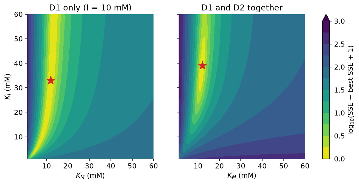
For D1, the landscape has a long, curved valley with an almost flat floor: the curve of constant \(K_M^\text{app}\) from the previous section. The grid point that happens to be lowest (\(K_M = 12\), \(K_I = 33\)) is no better than many others along the valley; 185 grid points come within one unit of the best SSE, with \(K_I\) anywhere from 2 to 60 mM. For D1 and D2 together, the valley closes into a basin with a single minimum, at \(K_M = 12\), \(K_I = 39\) on the grid, close to the least-squares estimate. The basin is still long in the \(K_I\) direction: grid points from 28 to 54 mM fit almost as well. \(K_I\) is identifiable from these data, although only loosely determined.
Grid search becomes hopeless quickly as parameters are added. Sixty values for each of two parameters makes 3600 evaluations; sixty values for each of ten parameters would make about \(6 \times 10^{17}\). This is the curse of dimensionality (book, §6.5.5), and it is why grid search is used for small problems, for a first look at a landscape, or to choose starting points for a local method.
4.4 Evolutionary algorithms
Between local methods, which are fast but need a good starting guess, and grid search, which is thorough but expensive, lie stochastic global methods such as simulated annealing and evolutionary algorithms (book, §6.3.4). Evolutionary algorithms borrow the logic of natural selection: a population of parameter sets is varied at random, and the better ones are more likely to survive into the next generation.
The algorithm below is one of the simplest of them, a (10 + 40) evolution strategy. It keeps 10 parent parameter sets. In each generation it makes 40 children by adding small random changes (“mutations”) to copies of randomly chosen parents, and the best 10 of all 50 become the next parents. The mutations shrink slowly from one generation to the next, so the search moves from exploring widely to refining locally. The parameters are searched on a logarithmic scale, which suits parameters whose plausible values span orders of magnitude.
Core MATLAB only.
%% A simple evolutionary algorithm for parameter estimation
% The same model and data as in fit_inhibition (D1 and D2 together), but
% now estimated by a (10 + 40) evolution strategy, which needs no starting
% guess and no gradients:
%   1. start from 50 random parameter sets and keep the best 10 (parents);
%   2. each generation, make 40 children, each a copy of a random parent
%      with small random changes to its parameters ('mutation');
%   3. keep the best 10 of parents and children; shrink the mutations a
%      little; repeat.
% Parameters are searched on a log scale, from 0.1 to about 316.
% Requires: core MATLAB only.

data = readmatrix(fullfile(sbp.data_dir(), 'competitive_inhibition.csv'));
S = [data(:, 1); data(:, 1)];
I = [10 * ones(20, 1); 20 * ones(20, 1)];
v = [data(:, 2); data(:, 3)];
delta = 0.1;
sse = @(log_p) sum(((10^log_p(1) * S ./ ...
    (10^log_p(2) * (1 + I / 10^log_p(3)) + S) - v) ./ (delta * v)) .^ 2);

rng(1);                            % fixed seed: the same run every time
lo = -1.0; hi = 2.5;               % bounds on log10 of each parameter
n_parents = 10; n_children = 40; n_generations = 60;
sigma = 0.5;                       % initial mutation size (log10 units)

% 1. Random start; keep the best 10
pop = lo + (hi - lo) * rand(50, 3);
cost = arrayfun(@(k) sse(pop(k, :)), (1:50)');
[~, order] = sort(cost);
parents = pop(order(1:n_parents), :);
parent_cost = cost(order(1:n_parents));
snapshots = {parents};
snapshot_gens = 0;
best_per_generation = zeros(1, n_generations + 1);
best_per_generation(1) = parent_cost(1);
n_evaluations = 50;

for g = 1:n_generations
    % 2. Children: mutated copies of randomly chosen parents
    pick = randi(n_parents, n_children, 1);
    children = parents(pick, :) + sigma * randn(n_children, 3);
    children = min(max(children, lo), hi);
    child_cost = arrayfun(@(k) sse(children(k, :)), (1:n_children)');
    n_evaluations = n_evaluations + n_children;
    % 3. Survival of the fittest, among parents and children together
    everyone = [parents; children];
    everyone_cost = [parent_cost; child_cost];
    [~, order] = sort(everyone_cost);
    parents = everyone(order(1:n_parents), :);
    parent_cost = everyone_cost(order(1:n_parents));
    sigma = sigma * 0.93;
    best_per_generation(g + 1) = parent_cost(1);
    if ismember(g, [5 20 n_generations])
        snapshots{end + 1} = parents; %#ok<SAGROW>
        snapshot_gens(end + 1) = g; %#ok<SAGROW>
    end
end

p = 10 .^ parents(1, :);
fprintf(['Best after %d generations (%d SSE evaluations): vmax = %.3f, ' ...
    'KM = %.3f, KI = %.3f, SSE = %.4f\n'], n_generations, n_evaluations, ...
    p(1), p(2), p(3), parent_cost(1));

%% Plot
fig = figure('Position', [100 100 1000 400]);
subplot(1, 2, 1)
semilogy(0:n_generations, best_per_generation, 'o-', ...
    'Color', [0.122 0.467 0.706], 'MarkerSize', 3);
hold on
yline(63.7765, '--', 'Color', [0.6 0.6 0.6]);
xlabel('Generation'); ylabel('Best SSE so far'); title('Convergence');
legend({'', 'least-squares optimum (fit\_inhibition)'}, 'Box', 'off');
box off

subplot(1, 2, 2)
colors = [0.733 0.733 0.733; 1.000 0.498 0.055;
          0.173 0.627 0.173; 0.122 0.467 0.706];
for k = 1:numel(snapshots)
    P = 10 .^ snapshots{k};
    loglog(P(:, 2), P(:, 3), 'o', 'Color', colors(k, :), ...
        'MarkerFaceColor', colors(k, :), 'MarkerSize', 5);
    hold on
end
xlim([0.1 316]); ylim([0.1 316]);
xlabel('K_M (mM)'); ylabel('K_I (mM)');
title('The 10 parents, as the search proceeds');
legend(compose('generation %d', snapshot_gens), 'Location', 'southeast', ...
    'Box', 'off');
box off
sbp.save_figure(fig, mfilename('fullpath'), 'fig-evolutionary');

results.best = struct('SSE', parent_cost(1), 'vmax', p(1), 'KM', p(2), ...
    'KI', p(3));
results.n_evaluations = n_evaluations;
results.best_per_generation = best_per_generation;
sbp.save_results(mfilename('fullpath'), results);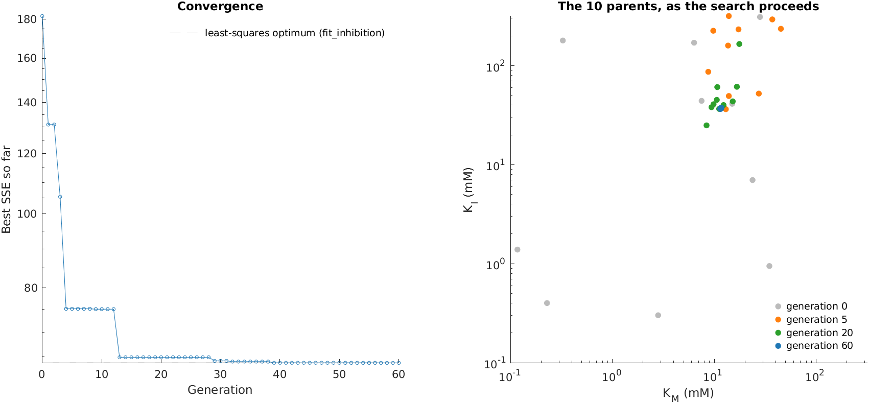
Needs NumPy and Matplotlib.
"""A simple evolutionary algorithm for parameter estimation.

The same model and data as in fit_inhibition (D1 and D2 together), but
now estimated by a (10 + 40) evolution strategy, which needs no starting
guess and no gradients:
  1. start from 50 random parameter sets and keep the best 10 (parents);
  2. each generation, make 40 children, each a copy of a random parent
     with small random changes to its parameters ('mutation');
  3. keep the best 10 of parents and children; shrink the mutations a
     little; repeat.
Parameters are searched on a log scale, from 0.1 to about 316.
"""
import numpy as np
import matplotlib.pyplot as plt
import sbp

data = np.loadtxt(sbp.DATA / "competitive_inhibition.csv", delimiter=",",
                  skiprows=1)
S = np.r_[data[:, 0], data[:, 0]]
I = np.r_[np.full(20, 10.0), np.full(20, 20.0)]
v = np.r_[data[:, 1], data[:, 2]]
delta = 0.1


def sse(log_p):
    vmax, KM, KI = 10.0 ** log_p
    v_pred = vmax * S / (KM * (1 + I / KI) + S)
    return np.sum(((v_pred - v) / (delta * v)) ** 2)


rng = np.random.default_rng(1)     # fixed seed: the same run every time
lo, hi = -1.0, 2.5                 # bounds on log10 of each parameter
n_parents, n_children, n_generations = 10, 40, 60
sigma = 0.5                        # initial mutation size (log10 units)

# 1. Random start; keep the best 10
pop = rng.uniform(lo, hi, size=(50, 3))
cost = np.array([sse(p) for p in pop])
keep = np.argsort(cost)[:n_parents]
parents, parent_cost = pop[keep], cost[keep]
snapshots = {0: parents.copy()}
best_per_generation = [parent_cost[0]]
n_evaluations = 50

for g in range(1, n_generations + 1):
    # 2. Children: mutated copies of randomly chosen parents
    pick = rng.integers(n_parents, size=n_children)
    children = parents[pick] + sigma * rng.standard_normal((n_children, 3))
    children = np.clip(children, lo, hi)
    child_cost = np.array([sse(p) for p in children])
    n_evaluations += n_children
    # 3. Survival of the fittest, among parents and children together
    everyone = np.vstack([parents, children])
    everyone_cost = np.r_[parent_cost, child_cost]
    keep = np.argsort(everyone_cost)[:n_parents]
    parents, parent_cost = everyone[keep], everyone_cost[keep]
    sigma *= 0.93
    best_per_generation.append(parent_cost[0])
    if g in (5, 20):
        snapshots[g] = parents.copy()
snapshots[n_generations] = parents.copy()

vmax, KM, KI = 10.0 ** parents[0]
print(f"Best after {n_generations} generations ({n_evaluations} SSE "
      f"evaluations): vmax = {vmax:.3f}, KM = {KM:.3f}, KI = {KI:.3f}, "
      f"SSE = {parent_cost[0]:.4f}")

# --- Plot
sbp.style()
fig, (ax1, ax2) = plt.subplots(1, 2, figsize=(10, 4))
ax1.semilogy(best_per_generation, "o-", color="#1f77b4", ms=3)
ax1.axhline(63.7765, color="#999999", ls="--",
            label="least-squares optimum (fit_inhibition)")
ax1.set_xlabel("Generation")
ax1.set_ylabel("Best SSE so far")
ax1.set_title("Convergence")
ax1.legend(frameon=False)

colors = {0: "#bbbbbb", 5: "#ff7f0e", 20: "#2ca02c", n_generations: "#1f77b4"}
for g, P in snapshots.items():
    ax2.plot(10.0 ** P[:, 1], 10.0 ** P[:, 2], "o", color=colors[g], ms=5,
             label=f"generation {g}")
ax2.set_xscale("log")
ax2.set_yscale("log")
ax2.set_xlim(0.1, 316)
ax2.set_ylim(0.1, 316)
ax2.set_xlabel("$K_M$ (mM)")
ax2.set_ylabel("$K_I$ (mM)")
ax2.set_title("The 10 parents, as the search proceeds")
ax2.legend(frameon=False, loc="lower right")
sbp.save_figure(fig, __file__, "fig-evolutionary")

sbp.save_results(__file__, {
    "best": {"SSE": parent_cost[0], "vmax": vmax, "KM": KM, "KI": KI},
    "n_evaluations": n_evaluations,
    "best_per_generation": best_per_generation,
})
sbp.show()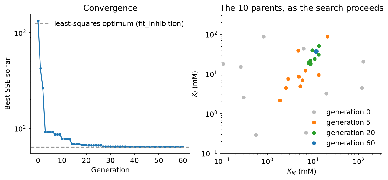
Starting from parameter sets scattered across more than three orders of magnitude, the population gathers into the basin we saw in the landscape and closes in on the least-squares estimate. After 60 generations, or 2450 evaluations of the SSE, the best parameter set is within a few per cent of the least-squares estimates, and its SSE is within 0.02% of the least-squares minimum. Notice that, on the way, the parents spread out along the same valley as before: the algorithm finds \(K_M^\text{app}\) well before it pins down \(K_M\) and \(K_I\) separately.
MATLAB and Python draw different random numbers, so the two versions follow different paths and end at slightly different points; the automated checks require both to land within 5% of the least-squares optimum. Run either version with a few different seeds to see how much the result varies.
The trade-off is clear from this small problem. The evolutionary algorithm needed no starting guess and no derivatives, but it used about 2450 evaluations to reach an approximate answer, whereas the least-squares solver reached the exact optimum in a few dozen evaluations, counting those used to estimate derivatives. For larger models, a common strategy is to combine the two: a global method to find the right basin, followed by a local method to finish the job.
4.5 Exercises
- Fit D2 alone from the eight starting points. Which combination of \(K_M\) and \(K_I\) do all the fits agree on?
- Fit D1 and D2 together using the unweighted SSE (book, Eq. 6.2). How do the estimates change, and which data points now dominate the fit?
- Estimate the uncertainty of the parameters fitted to D1 and D2 together. Both least-squares solvers return the Jacobian \(J\) of the residuals at the solution; the covariance of the estimates is approximately \((J^\top J)^{-1}\). Compute the correlation between \(K_M\) and \(K_I\) (book, Eq. 6.11). Is it close to \(\pm 1\)? Repeat for D1 alone: what happens to \(J^\top J\)?
- Book Exercise 6.1: evaluate the SSE of the parameter sets \(\theta_1\), \(\theta_2\) and \(\theta_3\) given there. Which is best, and can the data tell them apart?
- Run the evolutionary algorithm with ten different random seeds. How much do the final estimates vary? Then halve the number of generations, or start with a smaller mutation size, and repeat.
4.6 Going further
Here the model was a single algebraic rate law. Fitting a system of ODEs to time-course data works in exactly the same way, with the ODE solver of Chapter 3 called inside the residual function; the questions of identifiability and of local versus global search only become more pressing.