3 Dynamic models with ODEs
A dynamic model describes how the levels of molecules, such as metabolites, mRNAs or proteins, change over time. Most such models are systems of ordinary differential equations (ODEs),
\[ \frac{dx_i}{dt} = f_i(x_1, x_2, \ldots, x_n;\ \Theta), \qquad i = 1, 2, \ldots, n, \]
where \(x_i\) is the concentration of species \(i\), \(f_i\) is its rate law, and \(\Theta\) is the set of parameters, such as rate constants. This chapter covers the two halves of working with such models: writing the equations down, and solving them numerically, including what can go wrong.
Chapter 5, Introduction to Dynamic Modelling: mass-action kinetics (§5.2), enzyme kinetics and the Michaelis–Menten model (§5.3), solving ODEs (§5.5) and stiff equations (§5.6.1). Appendix E covers ODE solvers in MATLAB.
3.1 Solving an ODE: Euler’s method
Few ODE models can be solved on paper, so we solve them numerically. The simplest method, due to Euler, replaces the derivative by a finite difference over a small time step \(\Delta t\):
\[ x(t + \Delta t) \approx x(t) + f\big(x(t)\big)\,\Delta t . \]
Starting from the initial value \(x_0\), we step forward in time, one \(\Delta t\) at a time. This is the forward (or explicit) Euler method. The backward (or implicit) Euler method evaluates \(f\) at the end of the step instead, \(x(t + \Delta t) = x(t) + f\big(x(t + \Delta t)\big)\,\Delta t\), which must be solved for \(x(t + \Delta t)\) at every step.
We try both on an ODE with a known answer,
\[ \frac{dx}{dt} = a - bx, \qquad x(0) = c, \qquad x(t) = \frac{a}{b} - \left(\frac{a}{b} - c\right) e^{-bt}, \]
with \(a = 20\), \(b = 2\) and \(c = 5\), so \(x\) rises from 5 towards its steady state \(a/b = 10\).
Core MATLAB only.
%% Solving dx/dt = a - b*x with the forward and backward Euler methods
% This simple ODE has an exact solution, so we can see how the step size
% dt affects accuracy and, for forward Euler, stability.
% Requires: core MATLAB only.

a = 20; b = 2; c = 5;   % dx/dt = a - b*x,  x(0) = c
t_end = 4;
exact = @(t) a/b - (a/b - c) * exp(-b*t);

%% Forward Euler with different step sizes
steps = [0.05 0.25 0.9 1.1];
max_error = zeros(size(steps));
for k = 1:numel(steps)
    [t, x] = forward_euler(a, b, c, t_end, steps(k));
    max_error(k) = max(abs(x - exact(t)));
    fprintf('forward Euler, dt = %4g: max error = %.4g\n', ...
        steps(k), max_error(k));
end
fprintf('Forward Euler is stable only for dt < 2/b = %g\n', 2/b);

%% Forward vs backward Euler at a step size beyond the stability limit
[t_f, x_f] = forward_euler(a, b, c, t_end, 1.1);
[t_b, x_b] = backward_euler(a, b, c, t_end, 1.1);

%% Plot
colors = [0.122 0.467 0.706; 0.173 0.627 0.173;
          1.000 0.498 0.055; 0.839 0.153 0.157];
t_fine = linspace(0, 4.4, 441);
fig = figure('Position', [100 100 1000 400]);

subplot(1, 2, 1)
plot(t_fine, exact(t_fine), 'k-', 'LineWidth', 2);
hold on
for k = 1:3                     % dt = 1.1 is in the right panel
    [t, x] = forward_euler(a, b, c, t_end, steps(k));
    plot(t, x, 'o-', 'Color', colors(k, :), 'MarkerSize', 4);
end
ylim([0 20]);
xlabel('t'); ylabel('x(t)'); title('Forward Euler');
legend(['exact', compose('\\Deltat = %g', steps(1:3))], ...
    'Location', 'southeast', 'Box', 'off');
box off

subplot(1, 2, 2)
plot(t_fine, exact(t_fine), 'k-', 'LineWidth', 2);
hold on
plot(t_f, x_f, 'o-', 'Color', colors(4, :), 'MarkerSize', 4);
plot(t_b, x_b, 's-', 'Color', colors(1, :), 'MarkerSize', 4);
ylim([-2 25]);
xlabel('t'); title('Forward vs backward Euler');
legend({'exact', 'forward, \Deltat = 1.1', 'backward, \Deltat = 1.1'}, ...
    'Location', 'northwest', 'Box', 'off');
box off
sbp.save_figure(fig, mfilename('fullpath'), 'fig-euler');

results.steps = steps;
results.max_error_forward = max_error;
results.forward_dt_1_1 = x_f;
results.backward_dt_1_1 = x_b;
sbp.save_results(mfilename('fullpath'), results);

%% Local functions
function [t, x] = forward_euler(a, b, c, t_end, dt)
% x(t + dt) = x(t) + f(x(t)) * dt
n = round(t_end / dt);
t = dt * (0:n);
x = zeros(1, n + 1);
x(1) = c;
for i = 1:n
    x(i + 1) = x(i) + (a - b * x(i)) * dt;
end
end

function [t, x] = backward_euler(a, b, c, t_end, dt)
% x(t + dt) = x(t) + f(x(t + dt)) * dt, solved for x(t + dt).
% For a linear f this can be done by hand:
% x(t + dt) = (x(t) + a*dt) / (1 + b*dt).
n = round(t_end / dt);
t = dt * (0:n);
x = zeros(1, n + 1);
x(1) = c;
for i = 1:n
    x(i + 1) = (x(i) + a * dt) / (1 + b * dt);
end
end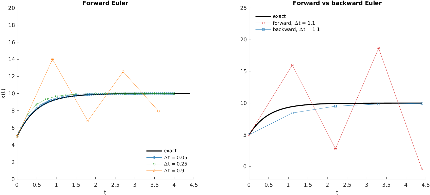
Needs NumPy and Matplotlib.
"""Solving dx/dt = a - b*x with the forward and backward Euler methods.

This simple ODE has an exact solution, so we can see how the step size
dt affects accuracy and, for forward Euler, stability.
"""
import numpy as np
import matplotlib.pyplot as plt
import sbp

a, b, c = 20, 2, 5      # dx/dt = a - b*x,  x(0) = c
t_end = 4


def exact(t):
    return a / b - (a / b - c) * np.exp(-b * t)


def forward_euler(dt):
    """x(t + dt) = x(t) + f(x(t)) * dt"""
    n = round(t_end / dt)
    t = dt * np.arange(n + 1)
    x = np.zeros(n + 1)
    x[0] = c
    for i in range(n):
        x[i + 1] = x[i] + (a - b * x[i]) * dt
    return t, x


def backward_euler(dt):
    """x(t + dt) = x(t) + f(x(t + dt)) * dt, solved for x(t + dt).

    For a linear f this can be done by hand:
    x(t + dt) = (x(t) + a*dt) / (1 + b*dt).
    """
    n = round(t_end / dt)
    t = dt * np.arange(n + 1)
    x = np.zeros(n + 1)
    x[0] = c
    for i in range(n):
        x[i + 1] = (x[i] + a * dt) / (1 + b * dt)
    return t, x


# --- Forward Euler with different step sizes
steps = [0.05, 0.25, 0.9, 1.1]
max_error = []
for dt in steps:
    t, x = forward_euler(dt)
    max_error.append(np.abs(x - exact(t)).max())
    print(f"forward Euler, dt = {dt:4}: max error = {max_error[-1]:.4g}")
print(f"Forward Euler is stable only for dt < 2/b = {2 / b}")

# --- Forward vs backward Euler at a step size beyond the stability limit
t_f, x_f = forward_euler(1.1)
t_b, x_b = backward_euler(1.1)

# --- Plot
sbp.style()
colors = ["#1f77b4", "#2ca02c", "#ff7f0e"]
t_fine = np.linspace(0, 4.4, 441)
fig, (ax1, ax2) = plt.subplots(1, 2, figsize=(10, 4))
ax1.plot(t_fine, exact(t_fine), "k-", lw=2, label="exact")
for dt, col in zip(steps[:3], colors):  # dt = 1.1 is in the right panel
    t, x = forward_euler(dt)
    ax1.plot(t, x, "o-", color=col, ms=4, label=f"Δt = {dt}")
ax1.set_ylim(0, 20)
ax1.set_xlabel("t")
ax1.set_ylabel("x(t)")
ax1.set_title("Forward Euler")
ax1.legend(frameon=False, loc="lower right")

ax2.plot(t_fine, exact(t_fine), "k-", lw=2, label="exact")
ax2.plot(t_f, x_f, "o-", color="#d62728", ms=4, label="forward, Δt = 1.1")
ax2.plot(t_b, x_b, "s-", color="#1f77b4", ms=4, label="backward, Δt = 1.1")
ax2.set_ylim(-2, 25)
ax2.set_xlabel("t")
ax2.set_title("Forward vs backward Euler")
ax2.legend(frameon=False, loc="upper left")
sbp.save_figure(fig, __file__, "fig-euler")

sbp.save_results(__file__, {
    "steps": steps,
    "max_error_forward": max_error,
    "forward_dt_1_1": x_f,
    "backward_dt_1_1": x_b,
})
sbp.show()
Small steps track the exact solution well, and the error shrinks roughly in proportion to \(\Delta t\). Large steps are a different matter. For this ODE, each forward Euler step multiplies the distance from the steady state by \((1 - b\,\Delta t)\). If \(\Delta t\) is between \(1/b\) and \(2/b\), this factor is negative but smaller than 1 in size, so the solution overshoots and oscillates, but still settles (\(\Delta t = 0.9\)). Beyond \(2/b = 1\) it is larger than 1 in size, and the solution oscillates with growing amplitude (\(\Delta t = 1.1\)): the method is unstable. Backward Euler multiplies the distance by \(1/(1 + b\,\Delta t)\) instead, which is less than 1 for any step size, so it stays stable even at \(\Delta t = 1.1\); it is merely inaccurate.
3.1.1 In practice: use a library solver
You will rarely write your own solver. MATLAB and SciPy provide well-tested solvers that choose the step size automatically to keep the estimated error within a tolerance you set. The main ones correspond closely:
| MATLAB | Python (SciPy) | |
|---|---|---|
| Call | [t, y] = ode45(f, tspan, y0, opts) |
sol = solve_ivp(f, t_span, y0, ...) |
| Right-hand side | f(t, y), returns a column vector |
f(t, y), returns a list or array |
| General-purpose (non-stiff) | ode45 |
method="RK45" (the default) |
| Lower accuracy, cheaper | ode23 |
method="RK23" |
| Stiff problems | ode15s, ode23s |
method="BDF", "Radau", or "LSODA" (switches automatically) |
| Tolerances | odeset('RelTol', 1e-6, 'AbsTol', 1e-9) |
rtol=1e-6, atol=1e-9 |
| Output at chosen times | pass a vector as tspan |
pass t_eval=... |
| Shape of the solution | y is time × species |
sol.y is species × time |
3.2 Enzyme kinetics: mass action vs Michaelis–Menten
For an enzyme \(E\) converting a substrate \(S\) into a product \(P\) through a complex \(ES\),
\[ E + S \underset{k_{-1}}{\overset{k_1}{\rightleftharpoons}} ES \xrightarrow{k_2} E + P , \]
mass-action kinetics gives one ODE per species, with \([E] = E_0 - [ES]\) because the total amount of enzyme is fixed (book, Eqs. 5.4 and 5.6). Assuming in addition that \([ES]\) changes slowly compared to \([S]\) (the quasi-steady-state approximation of Briggs and Haldane) collapses all of this into the familiar Michaelis–Menten rate law
\[ v = \frac{v_\text{max}[S]}{K_M + [S]}, \qquad v_\text{max} = k_2 E_0, \qquad K_M = \frac{k_{-1} + k_2}{k_1}. \]
The rate law is so widely used that it is easy to forget it is an approximation. The code below solves both models, for a small and a large amount of enzyme, with \(K_M = 2\) mM and \(S_0 = 10\) mM.
Core MATLAB only.
%% Full mass-action enzyme model vs the Michaelis-Menten rate law
%     E + S <-> ES -> E + P      (rate constants k1, k_1, k2)
% The full model tracks S, ES and P; the enzyme is E = E0 - ES. The
% Michaelis-Menten (Briggs-Haldane) approximation replaces all of this
% with a single rate law, v = vmax*S/(KM + S). How good is it?
% Requires: core MATLAB only.

k1 = 1.0; k_1 = 1.0; k2 = 1.0;     % 1/(mM s), 1/s, 1/s
KM = (k_1 + k2) / k1;              % Michaelis constant: 2 mM
S0 = 10.0;                         % initial substrate (mM)
opts = odeset('RelTol', 1e-8, 'AbsTol', 1e-10);  % tight tolerances

% Two cases: little enzyme (E0 << S0) and a lot of enzyme (E0 ~ S0)
names = {'low_enzyme', 'high_enzyme'};
E0s = [0.1 5.0];
t_ends = [150 6];

fig = figure('Position', [100 100 1000 400]);
for k = 1:2
    E0 = E0s(k);
    t = linspace(0, t_ends(k), 51);

    % Full model: y = [S; ES; P]
    full_model = @(t, y) [-k1*(E0 - y(2))*y(1) + k_1*y(2)
                          k1*(E0 - y(2))*y(1) - (k_1 + k2)*y(2)
                          k2*y(2)];
    [~, y] = ode45(full_model, t, [S0; 0; 0], opts);
    P_full = y(:, 3)';

    % Michaelis-Menten model: a single ODE for S
    vmax = k2 * E0;
    mm_model = @(t, S) -vmax * S / (KM + S);
    [~, S] = ode45(mm_model, t, S0, opts);
    P_mm = S0 - S';                % in the MM model, P = S0 - S

    err = max(abs(P_full - P_mm)) / S0;
    fprintf('E0 = %g mM: max |P_full - P_MM| = %.1f%% of S0\n', E0, 100*err);
    results.(names{k}) = struct('E0', E0, 't', t, 'P_full', P_full, ...
        'P_mm', P_mm, 'max_rel_difference', err);

    subplot(1, 2, k)
    plot(t, P_full, '-', 'Color', [0.122 0.467 0.706], 'LineWidth', 2);
    hold on
    plot(t, P_mm, '--', 'Color', [1.000 0.498 0.055], 'LineWidth', 2);
    xlabel('Time (s)'); ylabel('Product P (mM)');
    title(sprintf('E_0 = %g mM, S_0 = %g mM', E0, S0));
    legend({'full mass action', 'Michaelis–Menten'}, ...
        'Location', 'southeast', 'Box', 'off');
    box off
end
sbp.save_figure(fig, mfilename('fullpath'), 'fig-michaelis-menten');

sbp.save_results(mfilename('fullpath'), results);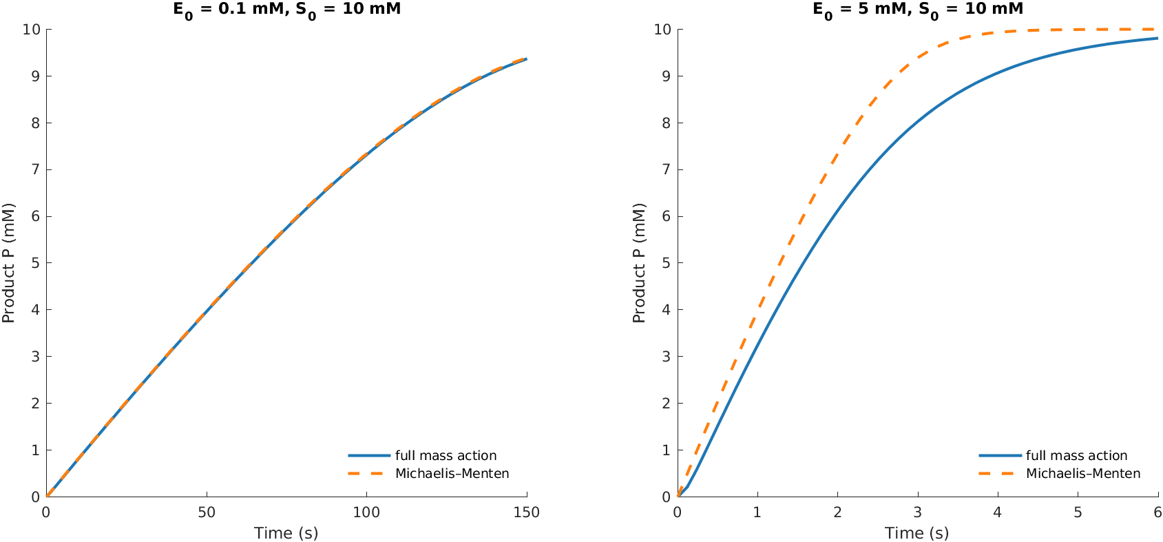
Needs SciPy.
"""Full mass-action enzyme model vs the Michaelis-Menten rate law.

    E + S <-> ES -> E + P      (rate constants k1, k_1, k2)

The full model tracks S, ES and P; the enzyme is E = E0 - ES. The
Michaelis-Menten (Briggs-Haldane) approximation replaces all of this
with a single rate law, v = vmax*S/(KM + S). How good is it?
"""
import numpy as np
from scipy.integrate import solve_ivp
import matplotlib.pyplot as plt
import sbp

k1, k_1, k2 = 1.0, 1.0, 1.0       # 1/(mM s), 1/s, 1/s
KM = (k_1 + k2) / k1               # Michaelis constant: 2 mM
S0 = 10.0                          # initial substrate (mM)
tol = dict(rtol=1e-8, atol=1e-10)  # tight tolerances for both solvers


def full_model(t, y, E0):
    """Mass-action ODEs for S, ES and P (book Eqs. 5.4)."""
    S, ES, P = y
    E = E0 - ES                    # enzyme conservation (Eq. 5.6)
    return [-k1 * E * S + k_1 * ES,
            k1 * E * S - (k_1 + k2) * ES,
            k2 * ES]


def mm_model(t, y, E0):
    """A single ODE for S, with the Michaelis-Menten rate law."""
    S = y[0]
    vmax = k2 * E0
    return [-vmax * S / (KM + S)]


def simulate(E0, t_end):
    t = np.linspace(0, t_end, 51)
    full = solve_ivp(full_model, [0, t_end], [S0, 0, 0], t_eval=t,
                     args=(E0,), **tol)
    mm = solve_ivp(mm_model, [0, t_end], [S0], t_eval=t, args=(E0,), **tol)
    P_full = full.y[2]
    P_mm = S0 - mm.y[0]            # in the MM model, P = S0 - S
    return t, P_full, P_mm


# Two cases: little enzyme (E0 << S0) and a lot of enzyme (E0 ~ S0)
cases = {"low_enzyme": (0.1, 150), "high_enzyme": (5.0, 6)}  # E0, t_end
results = {}
sbp.style()
fig, axes = plt.subplots(1, 2, figsize=(10, 4))
for ax, (name, (E0, t_end)) in zip(axes, cases.items()):
    t, P_full, P_mm = simulate(E0, t_end)
    err = np.abs(P_full - P_mm).max() / S0
    print(f"E0 = {E0} mM: max |P_full - P_MM| = {100 * err:.1f}% of S0")
    results[name] = {"E0": E0, "t": t, "P_full": P_full, "P_mm": P_mm,
                     "max_rel_difference": err}
    ax.plot(t, P_full, "-", color="#1f77b4", lw=2, label="full mass action")
    ax.plot(t, P_mm, "--", color="#ff7f0e", lw=2, label="Michaelis–Menten")
    ax.set_xlabel("Time (s)")
    ax.set_ylabel("Product P (mM)")
    ax.set_title(f"$E_0$ = {E0} mM, $S_0$ = {S0:g} mM")
    ax.legend(frameon=False, loc="lower right")
sbp.save_figure(fig, __file__, "fig-michaelis-menten")

sbp.save_results(__file__, results)
sbp.show()
With little enzyme, the two models are indistinguishable: they never differ by more than 0.3% of \(S_0\). With a lot of enzyme, the Michaelis–Menten model runs ahead of the full model by up to 14% of \(S_0\). The reason is that a substantial share of the substrate is held in the complex \(ES\), which the rate law ignores. A useful rule of thumb is that the approximation is good when \(E_0 / (S_0 + K_M) \ll 1\) (Segel and Slemrod 1989); here that ratio is 0.008 in the first case and 0.42 in the second. Know thy assumptions!
3.3 Stiff equations
The quasi-steady-state approximation works because binding is fast and catalysis is slow. That same separation of time scales causes trouble for numerical solvers. Below, the enzyme model is solved again with \(E_0 \ll S_0\), while binding and unbinding (\(k_1 = k_{-1}\)) are made faster and faster.
Core MATLAB only.
%% Stiffness: when fast binding makes a simple model expensive to solve
% The same enzyme model as before, but now binding and unbinding (k1, k_1)
% are much faster than catalysis (k2). The fast and slow time scales make
% the ODEs 'stiff'. We compare a non-stiff solver (ode45) with a stiff
% one (ode15s) by counting how often each one evaluates the right-hand
% side of the ODEs.
% Requires: core MATLAB only.

k2 = 1.0; E0 = 0.1; S0 = 10.0; t_end = 50.0;
opts = odeset('RelTol', 1e-6, 'AbsTol', 1e-9);

% y = [S; ES; P]
enzyme = @(t, y, k1, k_1) [-k1*(E0 - y(2))*y(1) + k_1*y(2)
                           k1*(E0 - y(2))*y(1) - (k_1 + k2)*y(2)
                           k2*y(2)];

%% How the cost grows as binding gets faster (k1 = k_1 = k)
speeds = [1 10 100 1000];
cost_nonstiff = zeros(size(speeds));
cost_stiff = zeros(size(speeds));
final_P = zeros(size(speeds));
for i = 1:numel(speeds)
    k = speeds(i);
    f = @(t, y) enzyme(t, y, k, k);
    nonstiff = ode45(f, [0 t_end], [S0; 0; 0], opts);
    stiff = ode15s(f, [0 t_end], [S0; 0; 0], opts);
    cost_nonstiff(i) = nonstiff.stats.nfevals;
    cost_stiff(i) = stiff.stats.nfevals;
    final_P(i) = stiff.y(3, end);
    fprintf(['k = %5g: ode45 used %7d evaluations, ode15s %5d;  ' ...
        'P(%g) = %.4f mM\n'], k, cost_nonstiff(i), cost_stiff(i), ...
        t_end, final_P(i));
end

%% The fast transient, for k = 100, on a logarithmic time axis
t = logspace(-4, log10(t_end), 41);
[~, y] = ode15s(@(t, y) enzyme(t, y, 100, 100), [0 t], [S0; 0; 0], opts);
y = y(2:end, :);               % drop t = 0, which we added as the start

%% Plot
fig = figure('Position', [100 100 1000 400]);
subplot(1, 2, 1)
semilogx(t, y(:, 2) / E0, '-', 'Color', [0.173 0.627 0.173], 'LineWidth', 2);
hold on
semilogx(t, y(:, 3) / S0, '-', 'Color', [0.122 0.467 0.706], 'LineWidth', 2);
xlabel('Time (s)'); ylabel('Fraction');
title('Two time scales (k_1 = k_{-1} = 100)');
legend({'ES / E_0 (fast)', 'P / S_0 (slow)'}, 'Location', 'northwest', ...
    'Box', 'off');
box off

subplot(1, 2, 2)
loglog(speeds, cost_nonstiff, 'o-', 'Color', [1.000 0.498 0.055]);
hold on
loglog(speeds, cost_stiff, 's-', 'Color', [0.122 0.467 0.706]);
xlabel('Binding rate constants k_1 = k_{-1}');
ylabel('Function evaluations');
title('Cost of solving to t = 50 s');
legend({'non-stiff solver', 'stiff solver'}, 'Location', 'northwest', ...
    'Box', 'off');
box off
sbp.save_figure(fig, mfilename('fullpath'), 'fig-stiff');

results.speeds = speeds;
results.final_P = final_P;
results.t = t;
results.ES_k100 = y(:, 2)';
results.P_k100 = y(:, 3)';
results.evaluations_nonstiff = cost_nonstiff;
results.evaluations_stiff = cost_stiff;
sbp.save_results(mfilename('fullpath'), results);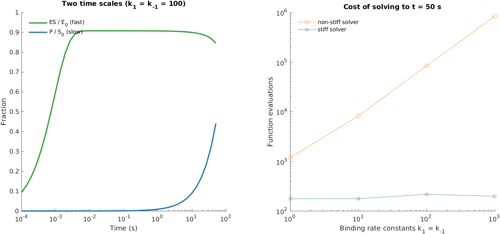
Needs SciPy.
"""Stiffness: when fast binding makes a simple model expensive to solve.

The same enzyme model as before, but now binding and unbinding (k1, k_1)
are much faster than catalysis (k2). The fast and slow time scales make
the ODEs 'stiff'. We compare a non-stiff solver (RK45, like ode45) with a
stiff one (BDF, like ode15s) by counting how often each one evaluates the
right-hand side of the ODEs.
"""
import numpy as np
from scipy.integrate import solve_ivp
import matplotlib.pyplot as plt
import sbp

k2, E0, S0, t_end = 1.0, 0.1, 10.0, 50.0
tol = dict(rtol=1e-6, atol=1e-9)


def enzyme(t, y, k1, k_1):
    S, ES, P = y
    E = E0 - ES
    return [-k1 * E * S + k_1 * ES,
            k1 * E * S - (k_1 + k2) * ES,
            k2 * ES]


# --- How the cost grows as binding gets faster (k1 = k_1 = k)
speeds = [1, 10, 100, 1000]
cost = {"nonstiff": [], "stiff": []}
final_P = []
for k in speeds:
    nonstiff = solve_ivp(enzyme, [0, t_end], [S0, 0, 0], method="RK45",
                         args=(k, k), **tol)
    stiff = solve_ivp(enzyme, [0, t_end], [S0, 0, 0], method="BDF",
                      args=(k, k), **tol)
    cost["nonstiff"].append(nonstiff.nfev)
    cost["stiff"].append(stiff.nfev)
    final_P.append(stiff.y[2, -1])
    print(f"k = {k:5}: RK45 used {nonstiff.nfev:7} evaluations, "
          f"BDF {stiff.nfev:5};  P({t_end:g}) = {stiff.y[2, -1]:.4f} mM")

# --- The fast transient, for k = 100, on a logarithmic time axis
t = np.logspace(-4, np.log10(t_end), 41)
sol = solve_ivp(enzyme, [0, t_end], [S0, 0, 0], method="BDF", t_eval=t,
                args=(100, 100), **tol)

# --- Plot
sbp.style()
fig, (ax1, ax2) = plt.subplots(1, 2, figsize=(10, 4))
ax1.semilogx(t, sol.y[1] / E0, "-", color="#2ca02c", lw=2,
             label="ES / $E_0$ (fast)")
ax1.semilogx(t, sol.y[2] / S0, "-", color="#1f77b4", lw=2,
             label="P / $S_0$ (slow)")
ax1.set_xlabel("Time (s)")
ax1.set_ylabel("Fraction")
ax1.set_title("Two time scales ($k_1 = k_{-1} = 100$)")
ax1.legend(frameon=False)

ax2.loglog(speeds, cost["nonstiff"], "o-", color="#ff7f0e",
           label="non-stiff solver")
ax2.loglog(speeds, cost["stiff"], "s-", color="#1f77b4",
           label="stiff solver")
ax2.set_xlabel("Binding rate constants $k_1 = k_{-1}$")
ax2.set_ylabel("Function evaluations")
ax2.set_title("Cost of solving to t = 50 s")
ax2.legend(frameon=False)
sbp.save_figure(fig, __file__, "fig-stiff")

sbp.save_results(__file__, {
    "speeds": speeds,
    "final_P": final_P,
    "t": t,
    "ES_k100": sol.y[1],
    "P_k100": sol.y[2],
    "evaluations_nonstiff": cost["nonstiff"],
    "evaluations_stiff": cost["stiff"],
})
sbp.show()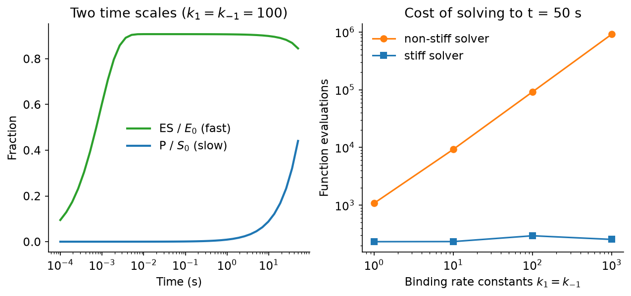
The left panel shows the two time scales: the complex \(ES\) forms within a few milliseconds, while the product takes tens of seconds to accumulate. After the first few milliseconds, nothing fast is happening, yet a non-stiff solver such as ode45 or RK45 must keep its steps small enough to remain stable with respect to the fast process, just as forward Euler had to keep \(\Delta t < 2/b\). Its cost therefore grows in proportion to the binding rate constants (right panel), reaching close to a million function evaluations. A stiff solver such as ode15s or BDF is implicit, like backward Euler, and can take large steps once the fast transient is over; its cost hardly changes. Both reach the same answer.
Such ODEs are called stiff: stability, rather than accuracy, limits the step size. Stiffness is common in biology, where binding, phosphorylation and transport often run much faster than gene expression or growth. A practical rule: start with ode45 or RK45, and if it is unexpectedly slow, switch to ode15s or BDF (or LSODA).
The exact counts differ between MATLAB and Python, because the solvers differ in their internals, but the pattern is the same; our automated checks compare only the solutions.
3.4 Exercises
- Run forward Euler with \(\Delta t = 1/b = 0.5\) and \(\Delta t = 2/b = 1\). Explain both results using the factor \((1 - b\,\Delta t)\).
- For the Michaelis–Menten example, vary \(E_0\) from 0.01 to 10 mM and plot the largest difference between the two models against \(E_0 / (S_0 + K_M)\).
- Make the product step reversible (\(E + P \to ES\) with rate constant \(k_{-2}\); book Eq. 5.3). Does the Michaelis–Menten rate law still describe the time course? What happens at long times?
- Solve the stiff example with \(k_1 = k_{-1} = 1000\) using
ode45andode15s(orRK45andBDF), timing each withtic/toc(ortime.perf_counter). - Replace the Michaelis–Menten rate law with a Hill rate law, \(v = v_\text{max}[S]^n / (K^n + [S]^n)\), and compare the time courses for \(n = 1, 2, 4\).
3.5 Going further
The parameters here were simply chosen. In practice, they must be estimated from data, which is the subject of the next chapter (book, Chapter 6).