NOSE — NOvel SpEcies Identification Pipeline
An automated, end-to-end Snakemake pipeline for novel microbial species identification and characterization from genomic assemblies, integrating fragmented manual workflows into a single, reproducible six-module pipeline.
What NOSE does
- Multi-metric novelty assessment — computes ANI (Average Nucleotide Identity), AAI (Average Amino Acid Identity), and POCP (Percentage of Conserved Proteins) against programmatically retrieved, validly published reference type strains, rather than relying on a single marker gene like 16S rRNA.
- Six-module Snakemake pipeline
- M1 – Quality & Identity Check: Genome quality assessment and taxonomic identification.
- M2 – Novelty Screening: ANI , AAI , POCP, and 16S analysis against reference type strains.
- M3 – Evolutionary Placement: Phylogenomic tree construction and evolutionary analysis.
- M4 – Metagenomic Mapping: Detects the prevalence and distribution of genomes across metagenomic datasets.
- M5 – Functional Profiling: Biosynthetic gene clusters, antimicrobial resistance genes, mobile genetic elements, and functional annotation.
- M6 – Metabolic Modeling: Genome-scale metabolic model reconstruction and pathway analysis.
- Browser-based GUI — a local browser-based interface (
nose-ui) for uploading genome assemblies, configuring module parameters, monitoring real-time logs, and running the pipeline with ease.
NOSE - Scientific Basis & Novelty Criteria
NOSE operates on standardized, empirically validated genomic boundaries to automatically identify and demarcate novel prokaryotic taxa. By integrating whole-genome relatedness indices (OGRIs) with species- and genus-level cutoff algorithms, the pipeline applies rigorous taxonomic criteria:
Species-Level Delineation (ANI < 95%)
- Algorithmic Basis: Average Nucleotide Identity (ANI) serves as the primary digital benchmark for species identification, directly replacing traditional, wet-lab DNA–DNA Hybridization (DDH).
- Empirical Threshold: An ANI value of ≥ 95–96% against standard reference strains indicates identity with a known species. Conversely, a pairwise ANI value < 95% across all available type strains provides robust mathematical proof of a novel species candidate.
- Supporting Literature:
- Konstantinidis & Tiedje (2005) established that the 95–96% ANI boundary directly corresponds to the classic 70% DDH species boundary.
- Jain et al. (2018) verified this threshold at scale using FastANI across >90,000 prokaryotic genomes, demonstrating an ultra-sharp biological gap between 95% and 98% ANI.
Genus-Level Delineation (POCP < 50%)
- Algorithmic Basis: Because ANI loses resolution at broader evolutionary distances, NOSE uses the Percentage of Conserved Proteins (POCP) metric to evaluate higher-rank taxonomic boundaries.
- Empirical Threshold: Pairwise shared protein content falling below 50% indicates significant evolutionary divergence, serving as the benchmark to demarcate a novel genus boundary.
- Supporting Literature:
- Qin et al. (2014) demonstrated that prokaryotic species within the same validly published genus share at least half of their protein content, establishing POCP < 50% as a robust standardized boundary for higher-level prokaryotic taxa.
Installation
NOSE is distributed as a Python package on PyPI and installed with pip. Each of its six modules runs in its own isolated Conda environment, deployed automatically by Snakemake at runtime — so you need a working Conda/Mamba installation on your system even though NOSE itself is a pip package.
System requirements
- Python 3.9 or newer
- A Conda distribution (Miniconda, Anaconda, or Micromamba) — required so Snakemake can build each module's environment with
--use-conda git, for cloning the repository (optional, if not installing from PyPI)curlorwget— used by the setup and database-download scripts to fetch tools and reference databases- Disk space — a few GB for NOSE and its conda environments, plus reference databases downloaded separately per module you actually run (GTDB-Tk ~66 GB, CheckM2 ~3 GB, antiSMASH/geNomad/COG a few GB each —
nose-dbchecks free space at the destination and warns you before each download) - A stable internet connection — needed for the initial pip/conda installs, database downloads, and live NCBI/GTDB lookups during Modules 1-3; a slow or dropped connection is the most common cause of a run that looks stuck rather than a real bug
- Input size — no hard limit on genome count, but runtime scales with it (Module 1's GTDB-Tk step usually dominates). For a first run, try a handful of genomes to confirm your setup works before pointing NOSE at a large batch
- A terminal to run commands in — Command Prompt, PowerShell, or Windows Terminal on Windows; Terminal.app on macOS; any shell on Linux. A code editor (VS Code, PyCharm, or similar) is optional but useful for editing
config.yamlfiles directly - Windows only: WSL2 with a distro named
Ubuntuinstalled — the actual bioinformatics tool runs are routed through it automatically;pip installand the web UI (nose-ui) work natively in PowerShell, butnose-setup/nose-dbneed a realbashon PATH
Note
Miniconda is the setup verified to work reliably on our lab HPC/server environment. If you hit solver or dependency conflicts with full Anaconda, switch to Miniconda.
Step 1 — Install Python (If Needed)
Every command on this page is typed into a terminal window, one line at a time: that's Command Prompt or PowerShell on Windows (search for either in the Start menu), Terminal on macOS (Cmd+Space, then type "Terminal"), or your Linux distribution's terminal application.
Linux — most distributions already ship Python. Check first, and only install it if this fails:
$ python3 --version
$ sudo apt update && sudo apt install python3 python3-pip
macOS — download the installer from python.org/downloads and run it, or install via Homebrew:
$ brew install pythonWindows — download the installer from python.org/downloads, run it, and check "Add python.exe to PATH" on the first screen before clicking Install.
Verify it worked in a new terminal window:
$ python3 --versionNote
This system Python is only needed to run the Conda installer in Step 2. NOSE itself always runs inside a dedicated Conda environment (created in Step 3 with Python 3.9 or newer) — you won't develop against this Python directly, and if you already have Conda installed, you can skip this step entirely since Conda bundles its own.
Step 2 — Install a Conda distribution
Select your platform, then a Conda distribution.
Verified working setup on our Linux HPC/server environment. Recommended if you have run into solver or dependency conflicts with full Anaconda.
# download and install Miniconda
$ wget https://repo.anaconda.com/miniconda/Miniconda3-latest-Linux-x86_64.sh
$ bash Miniconda3-latest-Linux-x86_64.sh
$ source ~/.bashrc
On a shared server, pin to the exact version we've verified against NOSE instead of "latest" (which changes over time and can shift behavior underneath you):
# pinned version verified on our lab server (Python 3.10)
$ curl -O https://repo.anaconda.com/miniconda/Miniconda3-py310_23.5.2-0-Linux-x86_64.sh
$ bash Miniconda3-py310_23.5.2-0-Linux-x86_64.sh
$ source ~/.bashrc
# download and install Anaconda
$ wget https://repo.anaconda.com/archive/Anaconda3-latest-Linux-x86_64.sh
$ bash Anaconda3-latest-Linux-x86_64.sh
$ source ~/.bashrcWarning
On some Linux HPC / shared-server setups, Anaconda's default channel priority or bundled package versions have caused solver conflicts when Snakemake builds NOSE's per-module environments. If that happens, switch to the Miniconda instructions above.
# install micromamba
$ "${SHELL}" <(curl -L micro.mamba.pm/install.sh)
$ source ~/.bashrc
Micromamba is a good option when you want conda-style environments without the overhead of a full Anaconda/Miniconda install — useful for constrained or containerized environments.
# Apple Silicon (M1/M2/M3)
$ curl -O https://repo.anaconda.com/miniconda/Miniconda3-latest-MacOSX-arm64.sh
$ bash Miniconda3-latest-MacOSX-arm64.sh

# Intel Mac
$ curl -O https://repo.anaconda.com/miniconda/Miniconda3-latest-MacOSX-x86_64.sh
$ bash Miniconda3-latest-MacOSX-x86_64.sh

$ source ~/.zshrc
Download the Anaconda macOS installer (.pkg) from anaconda.com/download and run it.
$ brew install micromambaNote
NOSE's module dependencies (Snakemake, FastANI, and the rest of the per-module bioinformatics tools) are Linux/macOS-first and are not reliably installable natively on Windows. We recommend using WSL (see the WSL tab) rather than native Windows for running NOSE.
- Download the Miniconda installer for Windows from docs.conda.io/en/latest/miniconda.html.
- Run the
.exeinstaller, keeping the default options. - Open Anaconda Prompt from the Start menu for the pip install step below.
- Download the Anaconda installer from anaconda.com/download and run it.
- Open Anaconda Prompt for the pip install step below.
WSL gives you a real Linux environment on Windows, which is what NOSE's module dependencies expect. This is the recommended path for Windows users.
- Open PowerShell as Administrator and run
wsl --install, then restart when prompted. This installs Ubuntu by default — no need to pick a distribution. - After restart, an Ubuntu terminal window opens automatically the first time (search "Ubuntu" in the Start menu after that). Follow the Linux → Miniconda instructions above inside it — the commands are identical inside WSL.
# inside the WSL Ubuntu terminal
$ wget https://repo.anaconda.com/miniconda/Miniconda3-latest-Linux-x86_64.sh
$ bash Miniconda3-latest-Linux-x86_64.sh
$ source ~/.bashrc
Step 3 — Install NOSE via pip
# create and activate an environment -- pip is listed explicitly since relying
# on python alone to pull it in isn't reliable across every conda channel
$ conda create -n nose python=3.9 pip -y
$ conda activate nose

# install NOSE from PyPI
$ pip install nose-pipeline
Step 4 — Configure environments & download reference databases
These commands are the CLI entry points exposed by the pip install:
# configure the per-module runtime conda environments
$ nose-setup

# bulk-download and index required reference databases
$ nose-db
Step 5 — Get an NCBI API key
Every module resolves organism names from GCA/GCF accessions via the NCBI Entrez API. A free API key raises the request rate limit and avoids throttling on large batches.
- Sign in (or create a free account) at ncbi.nlm.nih.gov/account.
- Open Account Settings → API Key Management and click Create an API Key.
- Copy the generated key.
Enter your NCBI email and API key once in the dashboard's Credentials section (or directly in nose_config.yaml) — it's picked up by all six modules automatically.
Note
The email is required; the API key is optional but strongly recommended — without it, NCBI limits requests to 3/second instead of 10/second, which slows down organism-name lookups on large batches.
Install from source
$ git clone https://github.com/RamanLab/NOSE.git
$ cd NOSE
$ pip install -e .
Verify the installation
$ nose-infoDisplays localized installation details and version control logs. If the command isn't found, confirm the environment you installed into is activated, and that its bin directory is on your PATH.
Usage & Tutorials
NOSE exposes four command-line entry points. Most day-to-day use goes through the browser GUI; the others handle setup and database management.
Command-line entry points
| Command | What it does |
|---|---|
nose-ui | Launches the browser-based GUI locally at http://localhost:5050 |
nose-setup | Configures the per-module runtime Conda environments |
nose-db | Bulk-downloads and indexes required reference databases |
nose-info | Displays localized installation details and version control logs |
Video Walkthrough
Watch the complete video tutorial on how to set up and navigate the NOSE pipeline and web interface.
Launching the browser UI
$ nose-uiOpens a local interface at http://localhost:5050 for uploading a genome assembly and steering each module's runtime parameters through per-module configuration panels. The frontend is plain HTML5/CSS3/vanilla JavaScript with no external framework, and pipeline logs stream to the browser in real time via Server-Sent Events.
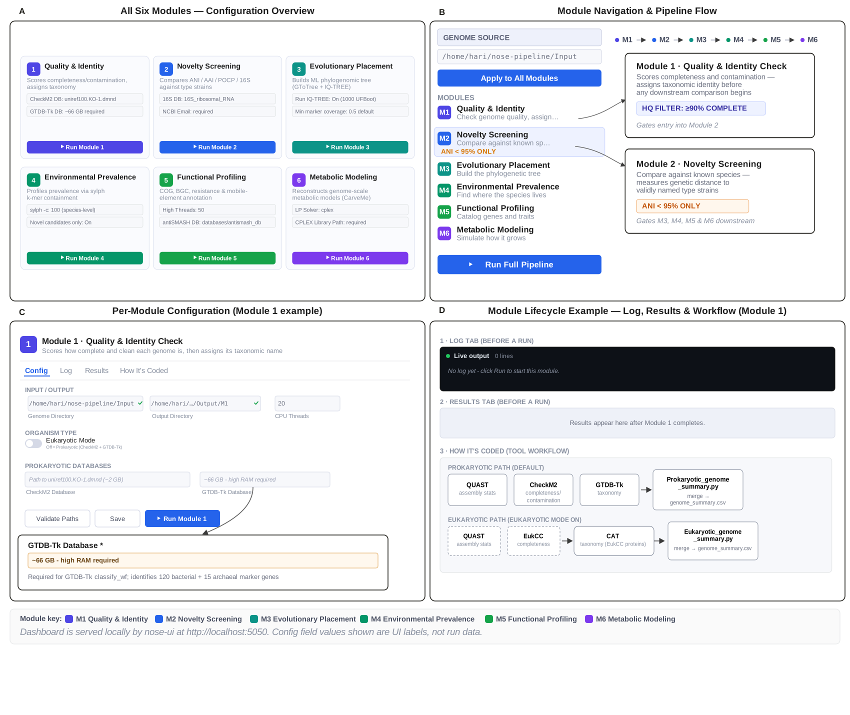
Controlling the UI
Use a different port — pass --port directly, or just run nose-ui with no flags: it checks whether 5050 is already taken and, if so, asks you for a port instead of failing outright.
# skip the interactive prompt and use a specific port directly
$ nose-ui --port 8080

# skip the prompt and accept the default (5050)
$ nose-ui --yes
Start without opening a browser tab — useful on a headless server, or when you're launching it from another script:
$ nose-ui --no-browser --yesCheck whether it's already running — the simplest check is just opening http://localhost:5050 (or whichever port you used) in a browser; if the dashboard loads, it's up. To check from the terminal instead, without opening anything:
# Windows (PowerShell)
$ Get-NetTCPConnection -LocalPort 5050 -ErrorAction SilentlyContinue

# macOS / Linux / WSL
$ lsof -i :5050
# or:
$ ss -tlnp | grep 5050
No output means nothing is listening on that port.
Stop it — if nose-ui is running in the foreground of the terminal you launched it from, Ctrl+C in that window stops it cleanly (this is exactly what the startup banner's "Ctrl+C to stop" line means). If it was started in the background, detached from a terminal, or you've lost track of which window it's in, stop it by port instead:
# Windows (PowerShell) -- finds and kills whatever owns port 5050
$ Get-NetTCPConnection -LocalPort 5050 -State Listen | Select-Object -ExpandProperty OwningProcess | ForEach-Object { Stop-Process -Id $_ -Force }

# macOS / Linux / WSL
$ lsof -ti:5050 | xargs kill -9
Note
A module runs as a child process of the dashboard, not a fully independent one -- so how you stop the dashboard matters. Ctrl+C in the same terminal window sends the interrupt to the whole process group, which will also stop a module that's actively running. Killing only the dashboard's own process by PID (the commands above) may leave an in-progress module running in the background rather than stopping it outright -- but the dashboard's own tracking of that run is only ever kept in memory, not on disk, so a freshly restarted nose-ui has no way to know it's still going and will show that module as idle again even if it's actually still working. To avoid the mismatch, either let a running module finish before restarting the dashboard, or click its Stop button in the UI first.
How a run flows
A single FASTA upload is passed through all six modules in sequence via a master dispatch script, which chains Snakemake sub-workflows together with custom Python/Bash post-processing. Every module reads its parameters from one centralized config.yaml, and each module's output is parsed into a standardized CSV/TSV that feeds directly into the next module.
Reading the output
Module 2 is the key novelty checkpoint: genomes with whole-genome ANI below 95% against the closest validly published reference are flagged as potential novel species and carried forward into phylogenomics, functional characterization, and metabolic modeling.
Every module writes a self-contained final_report.html alongside a "Download Excel" button and a full sortable/searchable data table for its results. Every chart in every report also has publication-quality export buttons — PNG, SVG, TIFF, EPS, and PDF, all rendered at a 300-DPI-equivalent scale — so a figure can go straight from a NOSE run into a manuscript without re-plotting it elsewhere.
Note
Step-by-step tutorials (example dataset, interpreting edge cases near the species boundary, customizing the reference genus lookup) will be added here.
Pipeline Details
NOSE is a Snakemake-based, six-module pipeline for detecting, classifying, and characterizing novel microbial species directly from genomic assemblies. Modules run sequentially, each in its own Conda environment, orchestrated by a master dispatch script around a centralized config.yaml.
Pipeline architecture
Data flow through all six modules — every tool, intermediate file, and hand-off between stages.
Module 1 Genome quality control & classification
Computes assembly metrics and taxonomic lineage for prokaryotic or eukaryotic input. Prokaryotes: QUAST for assembly stats, CheckM2 for completeness/contamination, GTDB-Tk (classify_wf) for taxonomy. Eukaryotes: QUAST, EukCC for completeness/redundancy, CAT (via MetaEuk-predicted proteins) against NCBI taxonomy. A unified High-Quality (HQ) filter — completeness ≥ 90%, contamination ≤ 5%, taxonomic resolution to at least Genus — gates what proceeds downstream; eukaryotic assemblies stop here and aren't propagated further.
Prokaryotic path (is_euk: false)
- QUAST — contig count, total length, GC%, N50/L50 assembly statistics
- CheckM2 — machine-learning
predictworkflow using the uniref100 database; accounts for lineage-specific marker gene presence and copy number - GTDB-Tk
classify_wf— identifies 120 bacterial + 15 archaeal marker genes to place genomes within the GTDB reference tree; confirms species-level ID via ANI against type strains Prokaryotic_genome_summary.py— parses GTDB classification into discrete taxonomic ranks and merges all outputs
Eukaryotic path (is_euk: true)
- QUAST — same assembly metrics as the prokaryotic path
- EukCC — single-genome mode with lineage-specific marker sets for completeness and redundancy estimation
- CAT — uses protein sequences predicted during the EukCC run (via the MetaEuk engine) for protein-level NCBI taxonomy classification; fragment bit-score cutoff (
-f) 0.5, r-value (-r) 3 Eukaryotic_genome_summary.py— merges outputs via outer joins on assembly identifiers
High-Quality (HQ) filter thresholds
Completeness   >= 90%    (CheckM2 or EukCC)
Contamination  <=  5%    (prokaryotes only)
Taxonomy: Domain through Genus must be fully resolved

Passes -> genome_summary.csv            -> feeds Module 2
Fails  -> unqualified_genome_summary.csv -> excluded
Key database requirement
GTDB-Tk requires a ~66 GB database. CheckM2 requires uniref100.KO.1.dmnd (~3 GB). Both must be pre-downloaded and their paths set in config.yaml before running.
Genome file extensions
.fasta, .fa, and .fna are all accepted interchangeably across every module — no need to rename files to match. Each module symlinks a .fasta-named entry alongside whichever extension your genomes actually use before processing starts.
Module 2 Genome-relatedness indices (OGRI)
Determines taxonomic position and genomic distance against validly published type strains, dynamically retrieved by genus. Computes three relatedness metrics in parallel — ANI (FastANI), AAI (aai.rb over Prokka-predicted proteomes), and POCP (Qin et al. 2014 method) — plus an optional 16S route via Barrnap + BLASTn. Genomes with WGS ANI < 95% are flagged as potential novel species and isolated for downstream phylogenomic validation.
FastANIaai.rbPOCPBarrnapBLASTnProkka16S rRNA workflow (is_16S: true)
- Input FASTA files with 16S sequences are queried against the NCBI 16S Ribosomal RNA Database using BLASTn
compile_results_16S.py— filters hits to the highest % identity per query, fetches NR/NG accessions and official organism names via Biopython Entrez- Output:
compiled_results.csvmapping each strain to its closest validly published relative with % identity and accession
WGS pipeline — 4 phases
- Phase 1 — 16S extraction: Barrnap predicts rRNA genes → BLASTn against the NCBI 16S DB identifies the host genus
- Phase 2 — Reference acquisition: NCBI TaxID retrieved → Datasets API queries all RefSeq (GCF) assemblies for that genus →
download_genomes.shbulk-downloads with verification and indexing - Phase 3 — ANI: FastANI compares each query against the full genus reference set; the best-matched reference (highest ANI) is identified for proteome-based steps
- Phase 4 — AAI + POCP:
aai.rbcomputes two-way AAI using reciprocal BLASTp (min 50 hits, 20% identity);pocp.shcalculates POCP per Qin et al. 2014 (40% aa identity, 50% coverage, E-value < 1×10⁻⁵)
Three genomic distance indices
- ANI — Average Nucleotide Identity: species-level boundary at 95%. Below = novel.
- AAI — Average Amino Acid Identity: assesses broader evolutionary distances via reciprocal BLASTp of Prokka-predicted proteomes
- POCP — Percentage of Conserved Proteins: genus-level delineation; < 50% suggests a different genus
compiled_results.csv output columns
Strain #             - query genome
Name (WGS)           - organism name (NCBI Entrez)
Accession # (WGS)    - best GCF reference
ANI (%)              - FastANI identity
AAI (%)              - two-way amino acid identity
PoCP%                - % conserved proteins
Name (16S)           - 16S rRNA best hit
Accession # (16S)    - NR accession
% similarities (16S) - BLASTn identity
Automatic outgroup & HMM-set selection for Module 3
As the last step of its own run, Module 2 resolves an outgroup genome and HMM set for every genus among the novel (ANI < 95%) candidates, writing them straight into genome_summary_for_tree.csv — Module 3 needs nothing filled in by hand for a normal run:
- HMM set — selected deterministically from the genome's GTDB phylum and class, no external lookup needed.
- Outgroup genome — resolved by trying progressively broader taxonomic ranks, and at each rank, progressively broader data sources. Starting at the genome's GTDB-Tk Order; if that's unresolved (common for genuinely novel, divergent genomes), moving to Class, then Phylum. At whichever rank is being tried, the GTDB REST API is queried first (authoritative type strains, no key required), falling back to an NCBI Entrez Assembly search at that same rank before widening further.
- A rank/genus combination already resolved in an earlier run is served from a local cache instead of re-querying — unless the cached result is itself empty (a past network failure), which always retries.
- If all three ranks come up empty, the genus is left with no outgroup and Module 3 skips that genus's tree entirely (an unrooted tree isn't useful).
Overriding the automatic choice
To use a different outgroup or HMM set for a genus, open genome_summary_for_tree.csv (Module 2's output) and edit the Outgroup and/or HMM cell for that genus's row directly, then run Module 3 — the column names must stay exactly Outgroup and HMM. This file is regenerated the next time Module 2 runs, so a hand-edit won't persist across reruns.
prepare_tree_inputs.py
Automatically isolates FASTA sequences and metadata for all ANI < 95% candidates, directly feeding Module 3 without manual file handling.
Decision Gate Novelty classification — ANI < 95%
A multi-metric taxonomic decision following established IJSEM standards. Isolates exhibiting ANI below 95% to their closest validly published relative are flagged as potential novel species and staged for downstream phylogenomic validation.
What each index contributes
- ANI (Average Nucleotide Identity) — primary species boundary. < 95% to any type strain = potential novel species
- AAI (Average Amino Acid Identity) — sensitive to broader evolutionary distances; corroborates ANI at the proteome level
- POCP (% Conserved Proteins) — genus-level boundary; < 50% POCP supports classification into a new genus
Output files written
compiled_results.csv   - all genomes (novel + known) with full OGRI metrics
potential_novel.csv    - ANI < 95% candidates only  -> feeds Module 3

prepare_tree_inputs.py auto-stages novel FASTA files
for phylogenomic tree construction
✦ ANI < 95% — candidate novel species: triggers the full M3–M6 characterization pipeline — M3 phylogenetics (GToTree + IQ-TREE confirms an isolated novel branch), M4 metagenomics (sylph profiles natural prevalence), M5 functional characterization, and M6 metabolic modeling.
✓ ANI ≥ 95% — known species: a full evidence table is still generated in compiled_results.csv, combining WGS and 16S identity metrics, organism name, and reference accession.
Module 3 Phylogenetic tree construction
Places genomes flagged as novel in Module 2 within their taxonomic context. Query genomes are partitioned into genus-specific clusters; conserved single-copy genes are extracted via genus-specific HMMs, and Maximum-Likelihood trees are inferred with bootstrap support. Outputs are formatted for interactive visualization. Genus grouping, HMM set, and outgroup are all filled in automatically by Module 2 — see its card above for how, and how to override it.
GToTreeIQ-TREEiTOLTwo-stage Snakemake workflow
- gtotree_snakefile — applies genus-specific HMMs via GToTree to extract universal Single-Copy Genes (SCGs); aligns and concatenates SCGs across query genomes, reference type strains, and the outgroup genome
- iqtree_snakefile — infers Maximum Likelihood trees using IQ-TREE on the concatenated SCG alignment; 1000 ultrafast bootstrap replicates for statistical branch support
IQ-TREE run command
iqtree \
  -s Aligned_SCGs.faa \   # concatenated SCG alignment
  -spp Partitions.txt \   # per-gene partition model
  -m MFP \                # ModelFinder Plus
  -bb 1000 \              # ultrafast bootstraps
  -nt 4 \                 # CPU threads
  -pre {genus}_iqtree_out # output prefix per genus
iTOL annotation — tree_annotation.py
- Generates per-genus annotation CSV files formatted for direct iTOL upload
- Colour-coded labels for novel candidate isolates, reference type strains, and the outgroup genome
- Bootstrap support values shown at internal nodes for assessment of novelty placement confidence
GToTree can silently exclude a genome
GToTree drops any genome recovering less than its -G completeness threshold (50% of expected marker genes by default) from the final tree. Module 3 detects this from GToTree's own removal log, warns per-genus, and writes Annotation/dropped_genomes_summary.csv listing which genomes were excluded and why. Set min_genome_coverage in Module 3's config to change the threshold — lower it to keep more genomes at the cost of less complete marker data.
Critical requirement
A genus with no resolved outgroup can't be rooted by GToTree and is skipped entirely — an unrooted tree is not useful, since branch support for novelty can't be correctly interpreted without one.
Module 4 Metagenomic Mapping Optional
Quantifies prevalence and relative abundance of novel species across user-provided metagenomic datasets using k-mer-based containment estimation — fast, and without the computational cost of read alignment. Produces a standardized master abundance table across samples.
Optional
Only runs if you provide raw metagenomic reads to screen against your novel genomes. If you don't have any, skip this module — the rest of the pipeline doesn't depend on it.
Detection thresholds used
containment threshold (c) = 100  ->  species-level resolution (default)
min-number-kmers          = 5    ->  mitigates false positives from
                                     low-complexity sequences

Alternative thresholds:
  c = 95  ->  genus-level
  c = 90  ->  family-level
Workflow steps
sylph_sketch_db— builds a.syldbsketch database once from all reference genomes (recursive FASTA scan)sylph_sketch_sample— sketches metagenomic reads: paired-end (_1/_R1+_2/_R2naming convention) viasylph sketch -1/-2, or single-end/unpaired reads viasylph sketch -rif no matching pair is foundsylph_profile— runs k-mer containment profiling at the set threshold against the reference sketch databasemerge_results.py— concatenates per-sample TSV outputs →final_report.csvwith aSample_IDcolumn added
final_report.csv output columns
- Sample_ID — metagenomic dataset identifier
- Genome — reference genome detected
- Containment — k-mer containment score
- ANI — estimated ANI derived from k-mer similarity
- Reads_Queried — total reads processed per sample
- Reads_Matching — reads matching the reference genome
Why sylph over alignment?
sylph uses k-mer containment estimation rather than base-by-base read alignment. No BAM files are generated and no reference index build is required — enabling rapid cross-sample profiling at scale.
Module 5 Functional characterization
Multi-modal profiling of genomic features, metabolic potential, resistance mechanisms, and mobile genetic elements: structural annotation and COG classification, secondary metabolite / biosynthetic gene cluster detection, prophage and plasmid identification, and antibiotic/biocide/metal resistance screening against curated databases. Results compile into summary tables for visualization.
ProkkaCOGclassifierantiSMASHgeNomadABRICATEStep 1 — Structural annotation
- Prokka identifies protein-coding sequences (CDS), ribosomal RNAs, and transfer RNAs via the Prodigal gene-finding algorithm
- Outputs per genome:
.gff(annotation),.faa(protein sequences),.ffn(nucleotide genes),.gbk(GenBank format)
Step 2–3 — COG functional classification
- COGclassifier classifies predicted proteins into Clusters of Orthologous Groups (COGs) against the NCBI Conserved Domain Database (CDD) — 26 functional categories
cog_merge.pypivots discrete classification counts into a comparative abundance matrix (merged_classifier_count.csv)
Step 4–5 — Secondary metabolite detection
- antiSMASH ("bacteria" taxon setting) detects Biosynthetic Gene Clusters: NRPS, PKS, terpenes, RiPPs, and more
--cb-generaland--cb-knownclustersflags enabled for comparison against the MIBiG databaseparserfile.py— custom HTML parsing engine extracts region coordinates, cluster types, and MIBiG similarity scores →AntiSMASH_results.csv
Step 6 — Resistance, virulence & biocide genes
- ABRICATE screens four curated databases: CARD (Antimicrobial Resistance), VFDB (Virulence Factors), BacMet2 (Biocide & Metal Resistance), NCBI
- High-confidence threshold: ≥ 80% nucleotide identity AND ≥ 80% query coverage enforced across all databases
Step 7 — Mobile element identification
- geNomad "end-to-end" mode predicts prophages and plasmids within each assembly
genomad_merge.pyconsolidates individual sample outputs → compiledvirus_summary.csv,virus_genes.csv,plasmid_summary.csv,plasmid_genes.csv
Why geNomad matters
ABRICATE tells you what resistance or virulence genes are present. geNomad tells you whether those genes reside on a mobile element (phage or plasmid) — meaning they have the capacity to spread horizontally to other organisms.
Module 6 Genome-scale metabolic model reconstruction Optional
Reconstructs a genome-scale metabolic model for each novel species via a top-down template approach, exported in standardized SBML/FBC format. Network topology and biomass connectivity are validated under unconstrained growth tests, and model quality is benchmarked for stoichiometric consistency.
Optional — requires your own CPLEX license
The default solver is IBM ILOG CPLEX, which needs a license you provide yourself — a free student/academic license works. If you don't have one, skip this module; it doesn't block anything else in the pipeline.
Getting CPLEX (student/academic license)
- Create an IBMid using your university/academic email address.
- Go to the IBM Academic Initiative downloads page and sign in.
- Select IBM ILOG CPLEX Optimization Studio.
- Search for "CPLEX 22.1.1" specifically — NOSE is verified against this version, not the older ones most generic install guides walk through.
- Choose the HTTP download option, then check the box for the installer matching your OS (e.g. "...CPLEX Optimization Studio V22.1.1 for Linux x86-64").
- Accept the license agreement — the Download button only appears once you do.
- Click Download. The installer file (e.g.
cplex_studio2211.linux-x86-64.bin) starts downloading.
Linux / macOS — make the installer executable and run it as superuser, accepting the default install path unless you have a reason to change it:
$ chmod +x cplex_studio2211.linux-x86-64.bin
$ sudo ./cplex_studio2211.linux-x86-64.bin
Windows — run the downloaded .exe installer as Administrator, keeping the default install path.
NOSE only needs the Python bindings
Unlike tools built against CPLEX's MATLAB bindings, NOSE calls CPLEX through its Python API. Once installed, that lives under the install directory at cplex/python/<python-version>/<platform> — for example:
/opt/ibm/ILOG/CPLEX_Studio2211/cplex/python/3.9/x86-64_linuxCopy that path into module6.cplex_lib_path in nose_config.yaml, or the CPLEX Library Path field on Module 6's Config tab (or the Full Pipeline Run page, under M6 settings). No environment variables or .bashrc edits needed — NOSE reads the path directly from config.
CarveMe reconstruction command
carve \
  --dna {genome.fasta} \   # DNA input mode
  --prodigal \             # high-fidelity gene prediction
  -o {sample}.sbml \       # SBML + FBC output
  --solver cplex \         # LP solver
  --diamond-args "-p {threads}"
Why --prodigal flag?
The --prodigal flag was specifically added to the pipeline after identifying that default gene prediction produced low gene counts for certain isolates, causing incomplete GEM reconstruction. Always keep this flag enabled.
LP solver options
CPLEX is NOSE's configured solver, as set up above. Gurobi is also supported as an alternative if you'd rather use a Gurobi license instead of CPLEX — set carveme.solver to gurobi in Module 6's config and point Gurobi License Path at your own installation instead of the CPLEX fields. Gurobi offers a free Named-User Academic license for eligible students and staff at gurobi.com/academia — activation (grbgetkey) needs to happen while on your institution's network or VPN.
Model validation — generate_model_stats.py
- COBRApy loads each SBML model and counts reactions, metabolites, and genes with metabolic function
- Unconstrained growth test: all exchange reaction bounds set to ±1000 mmol·gDW⁻¹·h⁻¹; biomass objective defined as the detected biomass reaction
growth = 0in the output indicates a disconnected or broken model requiring investigationcompile_model_summary.pyaggregates all individual model TSVs →model_summary.csvfor cross-isolate comparison
model_summary.csv columns
sample         - genome name
n_reactions    - total reactions in the GEM
n_metabolites  - total metabolites
n_genes        - genes with metabolic function
growth         - unconstrained max growth rate
               - 0 = model disconnected/broken
memote_score   - MEMOTE quality score (0-100%)
MEMOTE quality benchmarking
- Standardised quality control suite assessing stoichiometric consistency, metabolite formula redundancy, and mass/charge balance
- A MEMOTE snapshot HTML + JSON report is generated per isolate
- Scores cover multiple categories — a high overall score indicates a well-curated, publication-ready GEM
- GEMs exported in SBML/FBC format: compatible with COBRA Toolbox, cobrapy, cameo, OptFlux
Downloading a model
Module 6's HTML report has a "Download SBML" link next to each genome in its results table — the actual .sbml file CarveMe built, not just its summary stats, ready to open directly in COBRA Toolbox/cobrapy/etc.
Configuration & thresholds
| Module | Key threshold | How to change it |
|---|---|---|
| 1 — Quality control | Completeness ≥ 90%, contamination ≤ 5%, taxonomy resolved to ≥ Genus | Hardcoded in Module1/Prokaryotic_genome_summary.py (completeness_threshold, contamination_threshold) — edit those two variables directly, no config field for this yet |
| 2 — Relatedness | Novel candidate: WGS ANI < 95%; AAI ≥ 50 reciprocal hits at 20% identity; POCP ≥ 40% identity / 50% coverage / E-value < 1×10⁻⁵ | Hardcoded: ANI in Module2/compile_results_WGS.py and generate_report.py; AAI in Module2/aai.rb; POCP in Module2/pocp.sh — no config field for any of these three |
| 3 — Phylogenomics | Maximum-Likelihood tree, 1,000 ultrafast bootstrap replicates; genome kept in tree only if it recovers ≥ 50% of expected marker genes | Bootstrap count is hardcoded in Module3/iqtree_snakefile's -bb 1000 flag. The marker-gene threshold is a real config field — set min_genome_coverage in Module 3's config (or its Config tab in the dashboard) to something other than blank to override GToTree's 50% default |
| 4 — Mapping | Containment threshold (c) = 100, minimum 5 target k-mers per detection | The containment threshold is a config field — sylph_c in Module 4's config/Config tab (100 = species-level, 95 = genus-level, 90 = family-level). The minimum-k-mers value is hardcoded in Module4/snakefile |
| 5 — Annotation | Database matches ≥ 80% identity, ≥ 80% query coverage (CARD, VFDB, BacMet2, NCBI) | ABRICATE's own built-in defaults, not set explicitly anywhere in NOSE — to change them, add explicit --minid/--mincov flags to the run_abricate rule in Module5/snakefile |
| 6 — Metabolic models | Unconstrained growth test at ±1000 mmol·gDW⁻¹·h⁻¹ | Hardcoded in generate_model_stats.py's exchange-reaction bounds — no config field for this |
Config field vs. code edit
Only a few thresholds across the whole pipeline are exposed as actual config fields you can change from the dashboard without touching code: Module 3's min_genome_coverage and Module 4's sylph_c. Everything else in the table above is a value baked into the tool invocation or a post-processing script -- changing it means editing that specific file, then re-running the affected module (and redeploying if you're running from a server clone rather than editing in place). None of these are dangerous to change, but a code edit doesn't get picked up automatically the way a config field does.
Orchestration
Each module is a Snakemake sub-workflow running in its own Conda environment, deployed at runtime and chained together by a master dispatch script alongside custom Python/Bash connectors that standardize tool outputs into CSV/TSV between modules. A centralized config.yaml is the single point of control for analysis paths, parameter thresholds, and compute allocation.
Team & Credits
NOSE is developed at the Centre for Integrative Biology and Systems mEdicine (IBSE), Wadhwani School of Data Science and AI, IIT Madras.
- Prithvi S Prabhu
- Harippriya Sivakumar
- Enos Jadlin
- Pratyay Sengupta
- Karthik Raman — Principal Investigator
Acknowledgements
NOSE builds on open-source tools including FastANI, Snakemake, GTDB-Tk, CheckM2, and the other tools listed under Pipeline Details. See the repository for a full list of dependencies and licenses.
FAQ
Common questions about installing and running NOSE.
What counts as a "novel" species?
NOSE flags a genome as a novel candidate when its ANI to the closest reference genome falls below the species boundary threshold, given sufficient alignment coverage. A flagged result is a candidate for further taxonomic review, not a final classification.
Do I need my own reference database?
NOSE compares against whatever reference database you point it to. You can supply a custom set of reference genomes relevant to your organism group, or use a general-purpose reference set.
Can I run NOSE on a cluster?
Yes — since the pipeline is a Snakemake workflow underneath, it can be submitted to cluster or HPC schedulers using Snakemake's standard execution profiles.
Where do I report a bug or request a feature?
Open an issue on the NOSE GitHub repository.